Basic Reinforcement Learning
RL Setup
Env ------- s ------> Agent
 |     |--(r,s')-->|   |
 |                     |
 |<-------- a ---------|
MDP (Markov Decision Process): a classical formalization of sequential decision making, where actions influence subsequent situations or states
Env: the world with env dynamics where the agent lives and interacts, providing states \(s\) and rewards \(r\)
Agent: the learner or decision maker who produce actions \(a\) to the env, but cannot influence the dynamics \(p(s' \mid s,a)\) of the env
finite MDP: the sets of states \(s\), actions \(a\), and rewards \(r\) in a specific MDP all have a finite number of elements
Markov Property: the probability of each possible value for current state and reward: \(s_t,r_t\) depends only on the immediately preceding state and action: \(s_{t-1},a_{t-1}\)
in another words: the current state include information about all aspects of the past
6-tuple MDP: \((\mathcal{S}, \mathcal{A},p,\mathcal{R},\gamma,T)\)
\(s,s' \in \mathcal{S}\) - state space
\(a \in \mathcal{A}\) - action space
\(p (s' \mid s,a)\) - state transition probability (world model)
\(r (s,a,s') \in \mathcal{R}\) - reward function
\(\gamma \in [0,1)\) - discounting factor
\(T\) - horizon (can be finite or infinite)
Others:
\(\pi (a \mid s)\) - policy distribution gives action
\(t = 0,1,2,...,T\) - discrete time steps
\(h \triangleq [s_0,a_0,r_0,s_1,...,s_t,a_t,r_t,s_{t+1},...,s_T,a_T,r_T,s_{T+1}]\) - history trajectory (finite case)
\(R_t \triangleq \sum_{i=0}^{T} \gamma^i r_{t+i}\) - discounted return
Recursive Property:
\[\begin{align*} R_t &\triangleq r_t + \gamma r_{t+1} + \gamma^2 r_{t+2} + \gamma^3 r_{t+3} + ... \\ &= r_t + \gamma (r_{t+1} + \gamma r_{t+2} + \gamma^2 r_{t+3} + ...) \\ &= r_t + \gamma R_{t+1} \end{align*}\]Value Functions
Def: to evaluate how good it is for an agent to be in a given state in terms of future rewards that can be expected (Expected Return)
State-value function for policy \(\pi\): value function of a state \(s\) under a policy \(\pi\) is the expected return when starting in \(s\) and following \(\pi\) thereafter:
\[\begin{align*} V_{\pi}(s) &\triangleq \mathbb{E}_{\pi} \left[ R_t \mid s_t=s \right] \\ &= \mathbb{E}_{\pi} \left[ \sum_{i=0}^{T} \gamma^i r_{t+i} \mid s_t=s \right], \forall s \in \mathcal{S} \end{align*}\]Note:
-
\(V(s)\) can be changed due to different \(\pi\)
-
\(\mathbb{E}_{\pi}\) comes from the randomness of \(\pi\) and \(p(s' \mid s,a)\)
Action-value function for policy \(\pi\): the value of taking action \(a\) in state \(s\) under a policy \(\pi\) is the expected return starting from \(s\), taking the action \(a\) and following \(\pi\) thereafter:
\[\begin{align*} Q_{\pi}(s,a) &\triangleq \mathbb{E}_{\pi} \left[ R_t \mid s_t=s,a_t=a \right] \\ &= \mathbb{E}_{\pi} \left[ \sum_{i=0}^{T} \gamma^i r_{t+i} \mid s_t=s,a_t=a \right], \forall s \in \mathcal{S}, \forall a \in \mathcal{A} \end{align*}\]Bellman Equation of \(V_{\pi}\):
\[\begin{align*} V_{\pi}(s) &\triangleq \mathbb{E}_{\pi} \left[ R_t \mid s_t=s \right] \\ &= \mathbb{E}_{\pi} \left[ r_t+\gamma R_{t+1} \mid s_t=s \right] \\ &= \sum_a \pi(a \mid s) \sum_{s'} p(s' \mid s,a) \left[r_t+\gamma \mathbb{E}_{\pi} \left[R_{t+1} \mid s_{t+1}=s' \right] \right] \\ &= \sum_a \pi(a \mid s) \sum_{s'} p(s' \mid s,a) \left[r_t+\gamma V_{\pi}(s') \right] \\ &= \mathbb{E}_{\pi} \left[ r_t+\gamma V_{\pi}(s') \mid s_t=s \right], \forall s \in \mathcal{S} \end{align*}\]Meaning: the value of the start state must equal the discounted value of the expected next state plus the reward expected along the way
Backup Diagram:

update/backup operations: transfer value information back to a state or a state-action pair from its successor states or state-action pairs
Bellman Equation of \(Q_{\pi}\):
\[\begin{align*} Q_{\pi}(s,a) &\triangleq \mathbb{E}_{\pi} \left[ R_t \mid s_t=s,a_t=a \right] \\ &= \mathbb{E}_{\pi} \left[ r_t+\gamma V_{\pi}(s') \mid s_t=s,a_t=a \right] \\ &= \sum_{s'} p(s' \mid s,a) \left[ r_t+\gamma \mathbb{E}_{a' \sim \pi} Q_{\pi}(s',a') \mid s_{t+1}=s',a_{t+1}=a' \right] \\ &= \sum_{s'} p(s' \mid s,a) \left[ r_t+\gamma \sum_{a'} \pi(a' \mid s') Q_{\pi}(s',a') \mid s_{t+1}=s',a_{t+1}=a' \right], \forall s \in \mathcal{S}, a \in \mathcal{A} \end{align*}\]where
\[\begin{align*} V_{\pi}(s) &=\mathbb{E}_{a \sim \pi} Q_{\pi} (s,a) \\ &=\sum_{a \in \mathcal{A}} \pi(a \mid s) Q_{\pi} (s,a) \end{align*}\]Optimal Value Functions
Goal of RL: finding a policy that maximizes the expected return
Value functions define a partial ordering over policies:
a policy \(\pi\) is defined to be better than or equal to another \(\pi'\) for all states
\[\pi \geq \pi' \iff V_{\pi}(s) \geq V_{\pi'}(s), \forall s \in \mathcal{S}\]Optimal Policy \(\pi_*\): the policy that is better than or equal to all other policies
Optimal state-value and action-value function:
\[V_*(s) \triangleq \max_{\pi} V_{\pi}(s), \forall s \in \mathcal{S}\] \[Q_*(s,a) \triangleq \max_{\pi} Q_{\pi}(s,a), \forall s \in \mathcal{S}, \forall a \in \mathcal{A}\]therefore
\[Q_*(s,a) = \mathbb{E} \left[r_t + \gamma V_*(s') \mid s_t=s,a_t=a \right]\]Bellman Optimality Equations:
\[\begin{align*} V_*(s) &= \max_{a \in \mathcal{A}} Q_{\pi_*}(s,a) \\ &= \max_a \mathbb{E}_{\pi_*} \left[r_t + \gamma V_*(s') \mid s_t=s,a_t=a \right] \\ &= \max_a \sum_{s'} p(s' \mid s,a) \left[r_t +\gamma V_*(s') \right] \end{align*}\] \[\begin{align*} Q_*(s,a) &= \mathbb{E} \left[ {r_t+\gamma \max_{a'} Q_*(s',a') \mid s_t=s,a_t=a} \right]\\ &= \sum_{s'} p(s' \mid s,a) \left[r_t +\gamma \max_{a'} Q_*(s',a') \right] \end{align*}\]
the backup diagram is similar as before except that the arcs represent the maximum over the choices instead of taking expectation
Note:
-
Bellman optimality equation for \(V_*\) has a unique solution independent of \(\pi\)
-
if the dynamics \(p\) are known, the system equations w.r.t number of states of \(V_*\) can be solved
Once we have \(V_*\), we can determine \(\pi_*\):
-
any \(\pi\) assigns nonzero probability only to the actions where \(\max_a V_*(s)\) is obtained is \(\pi_*\)
-
any \(\pi\) that is greedy w.r.t \(V_*(s)\) is \(\pi_*\)
Policy Evaluation
\[\begin{align*} V_{k+1}(s) &\triangleq \mathbb{E}_{\pi} \left[r_t+ \gamma V_k(s_{t+1}) \mid s_t=s \right] \\ &=\sum_a \pi(a \mid s) \sum_{s'} p(s' \mid s,a) \left[r_t+\gamma V_k(s') \right], \forall s \in \mathcal{S} \end{align*}\]Note:
- \(V_k \rightarrow V_{\pi}\) is a fixed point for this update rule as \(k \rightarrow \infty\) because Bellman Equation for \(V_{\pi}\) assures us of equality in this case
Policy Improvement
Policy Improvement Theorem: Let \(\pi\) and \(\pi'\) be any pair of deterministic policies such that
\[\forall s \in \mathcal{S}, Q_{\pi}(s,\pi'(s)) \geq V_{\pi}(s)\]then the policy \(\pi'\) must be as good as or better than \(\pi\)
that is, it must obtain greater or equal expected return from all states \(s \in \mathcal{S}\):
\[V_{\pi'}(s) \geq V_{\pi}(s)\]Policy Improvement: the process of making a new policy that improves on an original policy, by making it greedy w.r.t the value function of the original policy
Define the new greedy policy \(\pi'\):
\[\begin{align*} \pi'(s) &\triangleq \arg \max_a Q_{\pi}(s,a) \\ &= \arg \max_a \mathbb{E} \left[r_t+\gamma V_{\pi}(s_{t+1}) \mid s_t=s,a_t=a \right] \\ &= \arg \max_a \sum_{s'} p(s' \mid s,a) \left[r_t+\gamma V_{\pi}(s') \right] \end{align*}\]Note:
- All the ideas can be easily generated to stochastic policies \(\pi(a \mid s)\)
Policy Iteration
The monotonical sequence of improving policies and value functions:
\(\pi_0\) -Evaluate-> \(V_{\pi_0}\) -Improve-> \(\pi_1\) -Evaluate-> \(V_{\pi_1}\) -Improve-> … \(\pi_*\) -Evaluate-> \(V_{\pi_*}\)
The process of Policy Iteration in deterministic policy case:
-
Policy Evaluation: \(V(s) \leftarrow \sum_{s'} p(s' \mid s,\pi(s)) \left[r+\gamma V(s') \right]\) until convergence
-
Policy Improvement: \(\pi(s) \leftarrow \arg \max_a \sum_{s'} p(s' \mid s,a) \left[r+\gamma V(s') \right]\) until policy being stable
Value Iteration
The Policy Evaluation step in Policy Iteration can be truncated without losing the convergence guarantees, which means we can do Policy Evaluation without waiting for the convergence of \(V_{\pi}\)
Value Iteration stops Policy Evaluation after just one update of each state
\[\begin{align*} V_{k+1}(s) &\triangleq \max_a \mathbb{E}_{\pi} \left[r_t+ \gamma V_k(s_{t+1}) \mid s_t=s \right] \\ &=\max_a \sum_{s'} p(s' \mid s,a) \left[r_t+\gamma V_k(s') \right], \forall s \in \mathcal{S} \end{align*}\]Another way of understanding Value Iteration is simply turning the Bellman Optimality Equation into an update rule
Recall Bellman Optimality Equation
\[V_*(s) = \max_a \sum_{s'} p(s' \mid s,a) \left[r_t +\gamma V_*(s') \right]\]The process of Value Iteration:
-
\(V(s) \leftarrow \max_a \sum_{s'} p(s' \mid s,a) \left[r+\gamma V(s')\right]\) until convergence
-
output a deterministic policy \(\pi(s)=\arg \max_a \sum_{s'} p(s' \mid s,a) \left[r+\gamma V(s')\right]\)
Monte Carlo Control
We consider action values \(Q_{\pi}(s,a)\) in Monte Carlo Control since Monte Carlo methods only uses experience samples without knowing the environment dynamics
The explicit estimate of value on each action is used to suggest a policy
a Monte Carlo version of Policy Iteration:
\(\pi_0\) -Evaluate-> \(Q_{\pi_0}\) -Improve-> \(\pi_1\) -Evaluate-> \(Q_{\pi_1}\) -Improve-> … \(\pi_*\) -Evaluate-> \(Q_{\pi_*}\)
-
Policy Improvement: \(\pi(s) \triangleq \arg \max_a Q(s,a)\) (by making the policy greedy w.r.t the current action value)
-
Policy Evaluation: \(Q(s,a) \leftarrow average(Returns(s,a))\) (run episode-by-episode)
Two assumptions for the guarantee of convergence for Monte Carlo method:
-
the episodes have exploring starts
-
policy evaluation could be done with an infinite number of episodes
On/Off Policy
To avoid the assumption of exploring starts:
On-policy methods: evaluate or improve the policy that is used to make decisions
Off-policy methods: evaluate or improve a policy different from that used to generate the data
In On-policy methods, the policy is generally soft, meaning \(\pi(a \mid s)>0, \forall s \in \mathcal{S}, a \in \mathcal{A}\) but gradually shifted closer to a deterministic optimal policy
\(\epsilon\)-greedy:
-
nongreedy action with probability of \(\frac{\epsilon}{\|\mathcal{A}(s)\|}\)
-
greedy action with probability of \(1-\epsilon+\frac{\epsilon}{\|\mathcal{A}(s)\|}\)
This form ensures any \(\epsilon\)-greedy policy w.r.t \(Q_{\pi}\) is an improvement under the policy improvement theorem
In a sense of exploration, on-policy methods learn action values not for the optimal policy, but for a near-optimal policy that still explores
Two-policy framework:
-
target policy: the policy being learned about and became optimal
-
behavior policy: the policy used to generate behavior for exploration
Off-policy: the process of learning from data ‘off’ the target policy
Comparison of On/Off-policy:
On-policy
(+) are generally simpler
(+) a special case of Off-policy methods that target and behavioral policies are the same
Off-policy
(-) require additional concepts and notation
(-) because the data is due to a different policy, they are often of greater variance and are slower to converges
(+) are more powerful and general
(+) can learn from data generated by a conventional non-learning controller, or from a human expert
(+) as key to learning multi-step predictive models of the world’s dynamics
Off-policy w/ Importance Sampling
Suppose we wish to estimate \(V_{\pi}\) and \(Q_{\pi}\), but all we have are episodes collected by another policy \(b\), where \(b \neq \pi\), in this case
-
\(\pi\) is the target policy
-
\(b\) is the behavior policy
and both are considered fixed and given
the assumption of coverage:
Every action taken under \(\pi\) is also taken, at least occasionally under \(\pi\), that is \(\pi(a \mid s)>0\) implies \(b(a \mid s)>0\)
Meaning: \(b\) must be stochastic in states where it is not identical to \(\pi\)
Importance Sampling: a general technique for estimating expected values under one distribution given samples from another
Importance Sampling Ratio: the relative probability of two trajectories occurring under the target and behavior policies
Given a starting state \(s_t\), the probability of the subsequent state-action trajectory occurring under any policy \(\pi\) is
\[\begin{align*} &P(a_t, s_{t+1},a_{t+1},s_{t+2},...,s_{T-1},a_{T-1},s_T \mid s_t,a_{t:T-1} \sim \pi) \\ &= \pi(a_t \mid s_t)p(s_{t+1} \mid s_t,a_t) \pi(a_{t+1} \mid s_{t+1})p(s_{t+2} \mid s_{t+1},a_{t+1}) ... \pi(a_{T-1} \mid s_{T-1})p(s_T \mid s_{T-1},a_{T-1}) \\ &= \prod_{k=t}^{T-1} \pi(a_k \mid s_k)p(s_{k+1} \mid s_k,a_k) \end{align*}\]Thus, the relative probability of the trajectory under the target and behavior policies (the importance-sampling ratio) is
\[\rho_{t:T-1} \triangleq \frac{\prod_{k=t}^{T-1} \pi(a_k \mid s_k)p(s_{k+1} \mid s_k,a_k)}{\prod_{k=t}^{T-1} b(a_k \mid s_k)p(s_{k+1} \mid s_k,a_k)} = \prod_{k=t}^{T-1} \frac{\pi(a_k \mid s_k)}{b(a_k \mid s_k)}\]Recall:
\[\mathbb{E}\left[R_t \mid s_t=s \right]=V_b(s)\]with the importance-sampling ratio:
\[\mathbb{E}\left[\rho_{t:T-1} R_t \mid s_t=s \right]=V_{\pi}(s)\]Off-policy Monte Carlo
We define
\(\mathcal{T}(s)\) for every-visit method - the set of all time steps in which state \(s\) is visited
\(\mathcal{T}(s)\) for first-visit method - only include time steps that were first visits to \(s\) within their episodes
\(T(t)\) - the first time of termination following time \(t\)
\(R(t)\) - the return after \(t\) up through \(T(t)\)
\(\{R(t)\}_{t \in \mathcal{T}(s)}\) - the returns that pertain to state \(s\)
\(\{\rho_{t:T(t)-1}\}_{t \in \mathcal{T}(s)}\) - the corresponding importance-sampling ratios
To estimate \(V_{\pi}(s)\), a simple average of the “ratio-ed” returns is Ordinary Importance Sampling:
\[V(s) \triangleq \frac{\sum_{t \in \mathcal{T}(s)} \rho_{t:T(t)-1} R(t)}{\|\mathcal{T}(s)\|}\]A weighted average is Weighted Importance Sampling:
\[V(s) \triangleq \frac{\sum_{t \in \mathcal{T}(s)} \rho_{t:T(t)-1} R(t)}{\sum_{t \in \mathcal{T}(s)} \rho_{t:T(t)-1}}\]Ordinary Importance Sampling
(+) unbiased
(-) unbounded variance because the variance of the ratios can be unbounded
(+) easier to extend to the approximate methods using function approximation
Weighted Importance Sampling
(-) biased (though the bias converges asymptotically to zero)
(+) lower variance (strongly prefer in practice)
Every-visit + both Ordinary and Weighted Importance Sampling
(-) biased
(+) remove the need to keep track of which states have been visited (preferred in practice)
(+) easier to extend to the approximate methods using function approximation (preferred in practice)
Episode-by-episode Incremental Monte Carlo:
Suppose we have a sequence of returns \(R_1,R_2,...,R_{n-1}\), all starting in the same state and each with a corresponding random weight \(W_i\) (e.g. \(W_i=\rho_{t_i:T(t_i)-1}\))
We wish to form the estimate
\[V_n \triangleq \frac{\sum_{k=1}^{n-1} W_k R_k}{\sum_{k=1}^{n-1} W_k}, n \geq 2\]and keep it up-to-date as we obtain a single additional return \(R_n\)
The update rule is
\[V_{n+1} \triangleq V_n + \frac{W_n}{C_n} \left[R_n - V_n \right], n \geq 1\] \[C_{n+1} \triangleq C_n + W_{n+1}\]Note of difference between first-visit and every-visit:
Exercise 5.5: an MDP with a single nonterminal state, a single terminal state and two actions

     --p-> s0 --(1-p)--> Terminal
     |     |
     |-----|

r +1 for all transitions
γ=1

Suppose you observe one episode that lasts 10 steps with a return of 10
What are the first-visit and every-visit estimators of the value of the nonterminal state?
first-visit: \(V(s)=10\)
every-visit: \(V(s)=(1/10)(1+2+3+4+5+6+7+8+9+10)=5.5\)
Important Concepts
Delayed reward:
Deterministic policy: \(\pi(s)\) always gives the exact same action for a given state
Stochastic policy: \(a \sim \pi(a \mid s)\) draws a sample from a distribution over actions when it encounters a state
Deterministic env: \(p(s' \mid s,a) = 1\)
Stochastic env: \(p(s' \mid s,a) \neq 1\)
Monte Carlo methods: only require experience samples to estimate \(V_{\pi}\) and \(Q_{\pi}\) by averaging over those samples and actual returns without knowing the model of env, and only for episodic tasks
Greedy: any search or decision procedure that selects alternatives based only on local or immediate considerations, without considering the possibility that such a selection may prevent future access to even better alternatives
Dynamic Programming: a collection of algs that can be used to compute optimal policies given a perfect model of the env as a MDP, and sometime require sweeps of the entire state set, (not applicable in practice but forms important theoretical foundations for RL algs)
Expected Update: all the updates done in DP is called Expected Update because they are based on an expectation over all possible next states rather than on a sample next state
Asynchronous DP: in-place iterative DP algs update the values of states in any order, using whatever values of other states happen to be available, other than algs sweep the entire state set of MDP
Generalized Policy Iteration: the general idea of letting Policy Evaluation and Policy Improvement process interact, independent of the granularity and other details of the two processes
A DP method is guaranteed to find an optimal policy in polynomial time w.r.t numbers of states and actions
DP vs Linear Programming vs direct search
Bootstrapping: algs update estimates on the basis of other estimates, like all of DP algs update estimates of \(V(s)\) based on estimates of \(V(s')\)
V(s) vs Q(s,a):
-
with a model, V(s) alone are sufficient to determine a policy; one simply looks ahead one step and chooses whichever action leads to the best combination of reward and next state
-
without a model, one must explicitly estimate the value of each action in order for the values to be useful in suggesting a policy
First-visit Monte Carlo: estimates \(V_{\pi}(s)\) as the average of the returns following first visits to \(s\)
Every-visit Monte Carlo: estimates \(V_{\pi}(s)\) as the average the returns following all visits to \(s\)
Exploring Starts: every (s,a) pair has a nonzero probability of being selected as the start
Gridworld
calculate Vπ

deterministic dynamics: p(s'|s,a)=1
actions={up,down,left,right}

r=+10, state A -> state A'
r=+5, state B -> state B'
r=-1, off the grid, location remains unchanged
r=0, otherwise

What is Vπ for π(a|s) ~ uniform with γ=0.9?
Solution is computed by solving the system of linear equations:
\[V_{\pi}(s)=\sum_a \pi(a \mid s) \sum_{s'} p(s' \mid s,a) \left[r+\gamma V_{\pi}(s') \right]\]since it’s a deterministic env, \(p(s' \mid s,a)=1\)
we have
\[V_{\pi}(s)=\sum_a \pi(a \mid s) \left[r+\gamma V_{\pi}(s') \right]\]for example from state \(s=(0,0)\) to \(s'\)
|   s   |   a   |   s'   |   r   |    |0,0|0,1|   |0,3|   |
|-------|-------|--------|-------|    |---|---|---|---|---|
|  0,0  | left  |  0,0   |  -1   |    |1,0|1,1|   |   |   |
|  0,0  |  up   |  0,0   |  -1   |    |---|---|---|---|---|
|  0,0  | right |  0,1   |  0    |    |   |   |   |2,3|   |
|  0,0  | down  |  1,0   |  0    |    |---|---|---|---|---|
                                      |   |   |   |   |   |
                                      |---|---|---|---|---|
                                      |   |4,1|   |   |   |
import numpy as np

nx,ny=5,5
A,A_=[0,1],[4,1]
B,B_=[0,3],[2,3]
actions=[[0,-1],[-1,0],[0,1],[1,0]]#left,up,right,down
pi=0.25
gm=0.9

def step(s,a):
    if s==A:
        return A_,10
    if s==B:
        return B_,5

    s_=[s[0]+a[0],s[1]+a[1]]
    if s_[0]<0 or s_[0]>=nx or s_[1]<0 or s_[1]>=ny:
        r=-1
        s_=s
    else:
        r=0

    return s_,r

V=np.zeros((nx,ny))

while True:
    V_=np.zeros_like(V)
    for x in range(nx):
        for y in range(ny):
            v_a=[]
            for a in actions:
                (x_,y_),r=step([x,y],a)
                v_a.append(pi*(r+gm*V[x_,y_]))
            V_[x,y]=np.sum(v_a)

    if np.sum(np.abs(V-V_))<1e-4:
        print(np.around(V,decimals=1))
        break

    V=V_
output:
[[ 3.3  8.8  4.4  5.3  1.5]
 [ 1.5  3.   2.3  1.9  0.5]
 [ 0.1  0.7  0.7  0.4 -0.4]
 [-1.  -0.4 -0.4 -0.6 -1.2]
 [-1.9 -1.3 -1.2 -1.4 -2. ]]
Insights:
-
negative values near the lower edge is due to the high probability of hitting the edge of the grid under the random policy
-
A is the best state to be under this policy
-
V(A)<10 because A’ is close to the edge and V(A’) has a negative value -1.3
-
V(B)>5 because V(B’) has a positive value 0.4
calculate V*
in this case, we don’t know the policy, and use \(max_a [r+\gamma V(s')]\) to update \(V\)
V=np.zeros((nx,ny))

while True:
    V_=np.zeros_like(V)
    for x in range(nx):
        for y in range(ny):
            v_a=[]
            for a in actions:
                (x_,y_),r=step([x,y],a)
                v_a.append(r+gm*V[x_,y_])
            V_[x,y]=np.max(v_a)

    if np.sum(np.abs(V-V_))<1e-4:
        print(np.around(V,decimals=1))
        break

    V=V_
output:
[[22.  24.4 22.  19.4 17.5]
 [19.8 22.  19.8 17.8 16. ]
 [17.8 19.8 17.8 16.  14.4]
 [16.  17.8 16.  14.4 13. ]
 [14.4 16.  14.4 13.  11.7]]
calculate Vk,π’,Vπ’

undiscounted episodic task (γ=1)
deterministic dynamics: p(s'|s,a)=1
actions={up,down,left,right}

terminal states: the shaded ones
non-terminal states: S={1,...,14}

r=-1, on all transitions until the terminal state is reached

if off the grid, location remains unchanged

What is {V_k} by iterative policy evaluation for π(a|s) ~ uniform?

What is Vπ' with π', where π' is an improved π?
-
\(\pi\) is the original equiprobable random policy
-
\(\pi'\) is the new policy greedy w.r.t \(V_{\pi}\)
-
we first obtained \(V_{\pi}\) with \(\pi\)
-
Then we replaced \(\pi\) with \(\pi'\), and calculate the new \(V_{\pi'}\)
-
\(V_{\pi'} \geq V_{\pi}\) because of policy improvement
Insights:
-
the state-value w.r.t a specific policy \(V_{\pi}\) converges to a fixed point can be referred to policy evaluation
-
a better policy greedily obtained from \(V_{\pi}\) can be referred to policy improvement
import numpy as np
import matplotlib.pyplot as plt

def is_terminal(s):
    return s==[0,0] or s==[nx-1,ny-1]

def step(s,a):
    if is_terminal(s):
        return s,0

    s_=[s[0]+a[0],s[1]+a[1]]

    if s_[0]<0 or s_[0]>=nx or s_[1]<0 or s_[1]>=ny:
        s_=s

    r=-1
    return s_,r

def plot_arrow(i,pi_op):
    scale=0.3
    x0=nx-0.5
    fig=plt.figure(figsize=(6,6))
    ax=fig.add_subplot(1,1,1)
    ax.set_aspect('equal', adjustable='box')
    ax.set_xticks(np.arange(0,nx+1,1))
    ax.set_yticks(np.arange(0,ny+1,1))
    plt.grid()
    plt.ylim((0,ny))
    plt.xlim((0,nx))

    for (x,y), label in pi_op.items():

        if [x,y]==[0,0] or [x,y]==[nx-1,ny-1]:
            pass
        else:
            if 1 in label: #up
                plt.arrow(y+0.5,x0-x,0,scale,width=0.1, head_width=0.2, head_length=0.1,fc='g', ec='g')
            if 3 in label: #down
                plt.arrow(y+0.5,x0-x,0,-scale,width=0.1, head_width=0.2, head_length=0.1,fc='c', ec='c')
            if 2 in label: #right
                plt.arrow(y+0.5,x0-x,scale,0,width=0.1, head_width=0.2, head_length=0.1,fc='b', ec='b')
            if 0 in label: #left
                plt.arrow(y+0.5,x0-x,-scale,0,width=0.1, head_width=0.2, head_length=0.1,fc='r', ec='r')
            plt.title('iteration:'+str(i))

    plt.savefig('policy_at_iter_'+str(i)+'.png',dpi=350)
    plt.show()
    plt.close()

def calc_vk(k=217,pi=0.25,gm=1):

    global nx,ny,actions
    nx,ny=4,4
    actions=[[0,-1],[-1,0],[0,1],[1,0]] #left, up, right, down

    V=np.zeros((nx,ny))
    pi_op={}

    for i in range(k):
        V_=np.zeros_like(V)

        for x in range(nx):
            for y in range(ny):
                v_a=[]
                for a in actions:
                    (x_,y_),r=step([x,y],a)
                    v_a.append(pi*(r+gm*V[x_,y_]))
                #policy evaluation
                V_[x,y]=np.sum(v_a)
                #obtain policy greedy w.r.t V_pi
                #policy improvement
                pi_op[x,y]=[i for i,v in enumerate(v_a) if v==max(v_a)]

        #convergence condition
        if np.sum(np.abs(V-V_))<1e-4:
            break

        V=V_

    plot_arrow(i,pi_op)

    return np.around(V,decimals=1),pi_op

def calc_v_improved(k,pi_op):
    V=np.zeros((nx,ny))

    for i in range(k):
        V_=np.zeros_like(V)

        for x in range(nx):
            for y in range(ny):
                v_a,pi=[0]*4,[0]*4
                for ia,a in enumerate(actions):
                    (x_,y_),r=step([x,y],a)
                    #apply improved policy
                    pi[ia]=1 if ia in pi_op[x,y] else 0
                    #policy evaluation with new policy
                    v_a[ia]=pi[ia]*(r+gm*V[x_,y_])
                V_[x,y]=np.sum(v_a)

        #convergence condition
        if np.sum(np.abs(V-V_))<1e-4:
            break

        V=V_

    return V

V_pi,pi_=calc_vk(k=217)
V_pi_=calc_v_improved(k=1,pi_op=pi_)
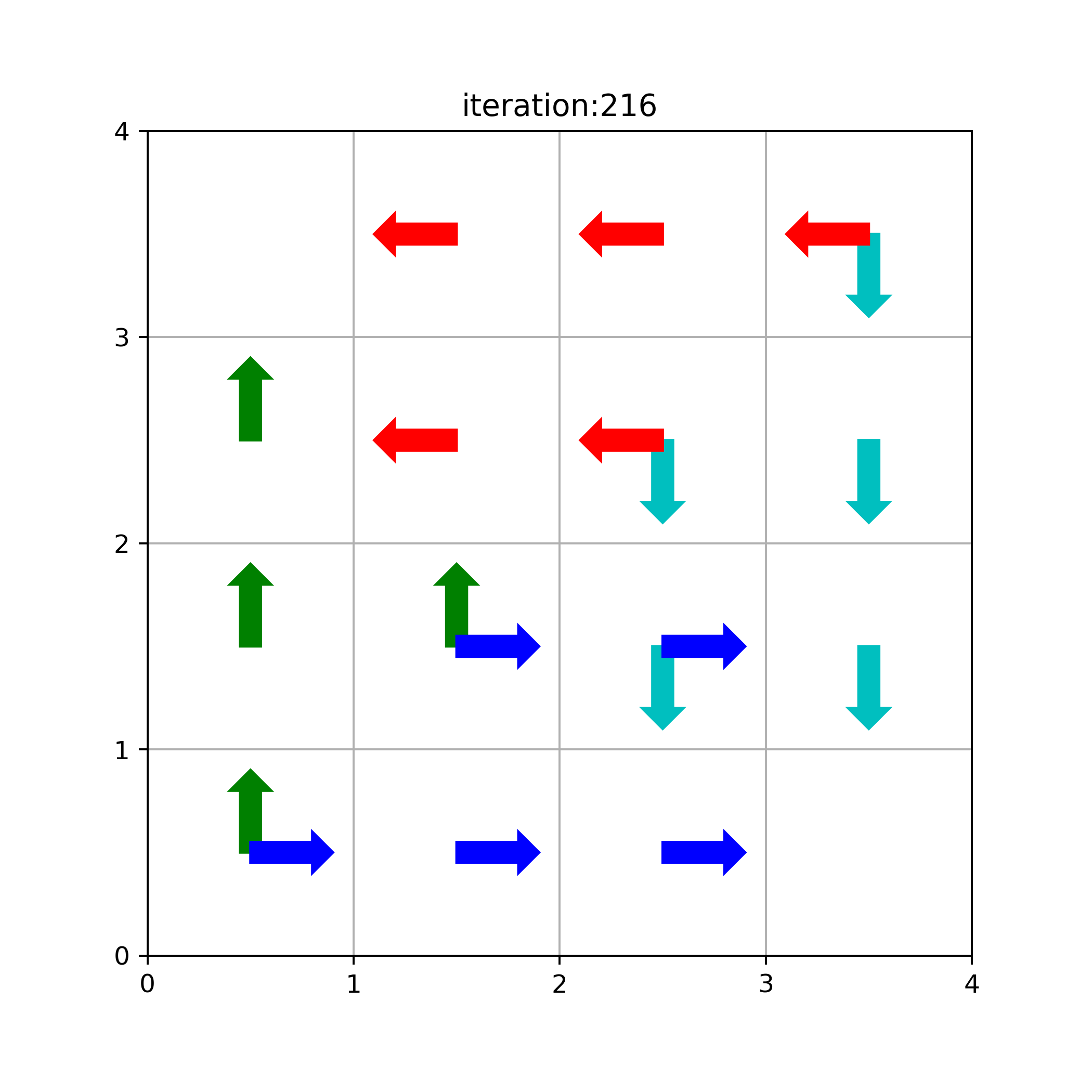
The above is the greedy policy we found at iteration 216, corresponding to Figure 4.1 k=216
V_pi=[[  0., -14., -20., -22.],
      [-14., -18., -20., -20.],
      [-20., -20., -18., -14.],
      [-22., -20., -14.,   0.]]

V_pi_=[[ 0., -1., -1., -2.],
      [-1., -1., -2., -1.],
      [-1., -2., -2., -1.],
      [-2., -1., -1.,  0.]]
Blackjack
Goal: to obtain cards the sum of whose numerical values is as great as possible without exceeding 21

face cards: 10
ace: 1 or 11
otherwise: same as the card number

Game begins with 2 cards dealt to both dealer and player

dealer's cards: one face up and one face down

player's cards:
    if immediately 21 (ace+10) <- natural: wins unless dealer also has a natural (draw)
    if not natural: can request additional cards one by one (hits) until he either stops (sticks) or exceeds 21 (goes bust)
        if goes bust: lose
        if sticks: then dealer's turn

dealer's policy: sticks on any sum of 17 or greater, and hits otherwise
    if goes bust: lose

the outcome is determined by the closeness to 21 of each one's final sum

if the player holds an ace that he could count as 11 without going bust, then the ace is said to be usable

---------------------------------------------------------------------------

an episodic undiscounted finite MDP (one game one episode, γ=1)

r=+1 win
r=-1 lose
r=0 draw

states: [player's sum, dealer's card, usable ace?], 10x10x2=200
    the player's current sum (12-22)
    the dealer's one showing card (A-10)
    whether or not the player holds a usable ace (True/False)

actions: [hit, stick]

policy:
    sticks, if the player's sum is 20 or 21
    hits, otherwise

episode 1:
    dealer's card: J
    player's hand: 9,Q
    player's action: hit
    player's hand: 9,Q,3, r=-1

    s=[19,10,no], a=[hit], s'=[22,10,no], r=-1

episode 2:
    dealer's card: J,3,9
    player's hand: 3,Q,3,3

    s=[13,10,no], a=[hit], s'=[16,10,no], r=0
    s=[16,10,no], a=[hit], s'=[19,10,no], r=0
    s=[19,10,no], a=[hit], s'=[19,22,no], r=1

    V(13,10,no) <- 1
    V(16,10,no) <- 1
    V(19,10,no) <- -1+1
first-visit Monte Carlo
for every episode:
- generate episode trajectory \([s_0,a_0,r_0,s_1,a_1,r_1,...,s_T,a_T,r_T]\) following \(\pi\)
- for each first appeared state \(s_{first}\): \(Q=\sum_{s \in [s_{first}:]} r\gamma^i\)
- append \(Q\) to return \(R(s)\)
- calculate the average: \(V(s) \leftarrow average(R(s))\)
The following code (based on this work) uses first-visit MC to approximate \(V(s)\) for the blackjack policy that sticks only on 20 or 21
import gym
import numpy as np
import matplotlib.pyplot as plt
from mpl_toolkits.mplot3d import Axes3D
from collections import defaultdict

plt.style.use('ggplot')

env=gym.make('Blackjack-v1')

#policy: hit until reach 20
#actions: 0-stick, 1-hit
def sample_policy(s):

    player_card, _, _ = s
    return 0 if player_card >= 20 else 1

def first_visit_mc(policy,env,n_eps,gm=1):

    ret_sum=defaultdict(float)
    ret_cnt=defaultdict(float)
    V=defaultdict(float)

    for ep in range(n_eps):
        traj,done=[],False
        s=env.reset()

        while not done:
            a=policy(s)
            s_,r,done,_=env.step(a)

            traj.append((s,a,r))
            s=s_

        #get unique states
        ss=set([t[0] for t in traj])

        for i, s in enumerate(ss):

            #find first occurence of each unique state
            idx=traj.index([t for t in traj if t[0]==s][0])

            #sum up all the discounted rewards starting from the first occurence
            Q=sum([t[2]*gm**i for t in traj[idx:]])

            ret_sum[s]+=Q
            ret_cnt[s]+=1.0
            V[s]=ret_sum[s]/ret_cnt[s]

    return V

def plot_blackjack(V,ax1,ax2):
    player_sum=np.arange(12,21+1)
    dealer_show=np.arange(1,10+1)
    usable_ace=np.array([True,False])

    vs=np.zeros((len(player_sum),len(dealer_show),len(usable_ace)))

    for i, p in enumerate(player_sum):
        for j, d in enumerate(dealer_show):
            for k, ace in enumerate(usable_ace):
                vs[i,j,k]=V[p,d,ace]

    X,Y=np.meshgrid(player_sum,dealer_show)

    ax1.plot_wireframe(X,Y,vs[:,:,0])
    ax2.plot_wireframe(X,Y,vs[:,:,1])

    for ax in ax1,ax2:
        ax.set_zlim(-1,1)
        ax.set_ylabel('player sum')
        ax.set_xlabel('dealer card')
        ax.set_zlabel('V(s)')

V_10000=first_visit_mc(sample_policy,env,n_eps=10000)
V_500000=first_visit_mc(sample_policy,env,n_eps=500000)

fig,axes=plt.subplots(nrows=2,ncols=2,figsize=(8,8),subplot_kw={'projection': '3d'})

axes[0,0].set_title('After 10000 episodes \n V(s) usable ace')
axes[1,0].set_title('V(s) no usable ace')
axes[0,1].set_title('After 500000 episodes \n V(s) usable ace')
axes[1,1].set_title('V(s) no usable ace')

plot_blackjack(V_10000,axes[0,0],axes[1,0])
plot_blackjack(V_500000,axes[0,1],axes[1,1])
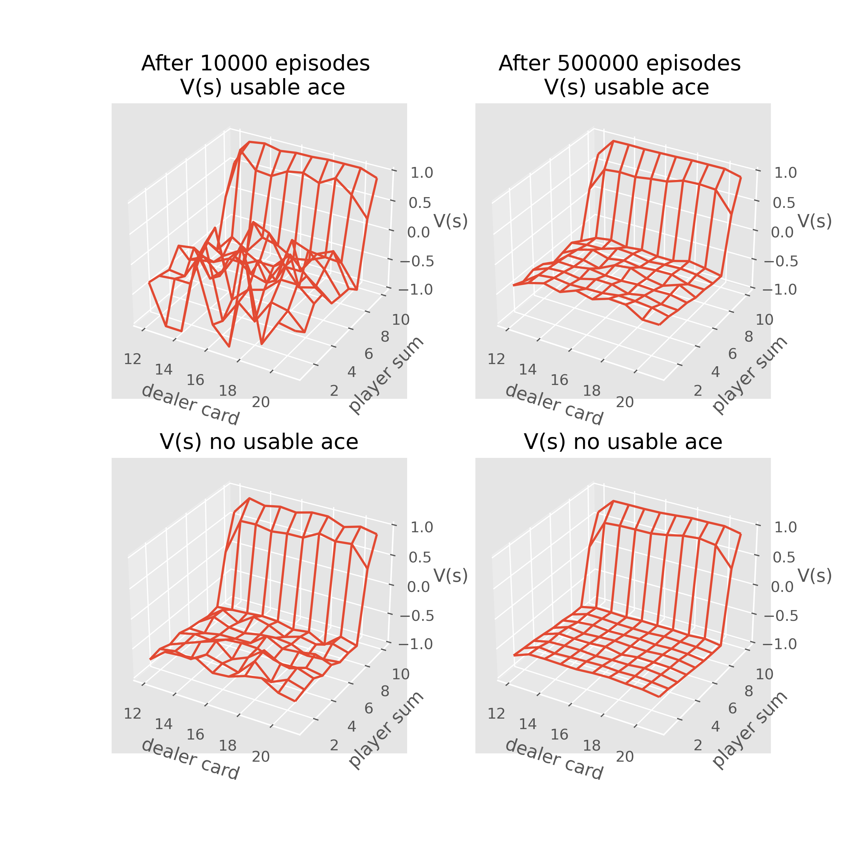
The above corresponds to Figure 5.1
Insights:
-
the estimates for states with a usable ace are less certain and less regular because these states are less common
-
there is only a small winning rate no matter what the number the dealer’s holding and what the player’s sum is for the policy: hit until reach 20
Monte Carlo Exploring Start
-
use random initialization for state and action
-
use greedy policy: \(a=\arg\max_a Q(s,a)\)
-
maintain Q(s,a) with state-action pairs instead of V(s) in the previous method
def mc_es(env,n_eps,gm=1.0):

    ret_sum=defaultdict(float)
    ret_cnt=defaultdict(float)

    na=env.action_space.n
    Q=defaultdict(lambda: np.zeros(na))

    for ep in range(n_eps):
        traj=[]
        s=env.reset() #random initial state
        a=np.random.randint(na) #random initial action

        for i in range(100):

            if i==0:
                pass
            else:
                #greedy policy w.r.t Q[s]
                a=np.random.choice([a for a,q in enumerate(Q[s]) if q==np.max(Q[s])])

            s_,r,done,_=env.step(a)
            traj.append((s,a,r))

            if done:
                break

            s=s_

        # find the unique state-action pairs
        pairs=set([(t[0],t[1]) for t in traj])

        for (s,a) in pairs:

            pair=(s,a)
            # find the first occurence of each state-action pair
            idx=traj.index([t for t in traj if t[0]==s and t[1]==a][0])
            V=sum([t[2]*gm**i for i, t in enumerate(traj[idx:])])

            ret_sum[pair]+=V
            ret_cnt[pair]+=1.

            Q[s][a]=ret_sum[pair]/ret_cnt[pair]

    V=defaultdict(float)
    for s, a_s in Q.items():
        V[s]=np.max(a_s)

    return Q,V

def plot_policy(Q):

    player_sum=np.arange(21,11,-1)
    dealer_show=np.arange(1,10+1)

    X,Y=np.meshgrid(dealer_show,player_sum)

    pi_ace=np.zeros((len(dealer_show),len(player_sum)))
    pi_noace=np.zeros((len(dealer_show),len(player_sum)))

    for (p,d,ace),q in Q.items():
        if ace==1:
            pi_ace[21-p,d-1]=np.argmax(q)
        elif ace==0 and p>11:
            pi_noace[21-p,d-1]=np.argmax(q)

    fig=plt.figure(figsize=(10,6))
    x_ticks_labels = ['A','2','3','4','5','6','7','8','9','10','11']
    y_ticks_labels = ['21','20','19','18','17','16','15','14','13','12','11']

    ax1=fig.add_subplot(1,2,1)
    ax1.set_aspect('equal', adjustable='box')
    ax1.set_xticks(np.arange(0,11,1))
    ax1.set_yticks(np.arange(0,11,1))
    ax1.set_xticklabels(x_ticks_labels)
    ax1.set_yticklabels(y_ticks_labels)
    plt.grid()
    im1=plt.imshow(pi_ace,cmap='gray_r')
    plt.colorbar(im1,fraction=0.046, pad=0.04)
    plt.title('$\pi_*$ usable ace')

    ax2=fig.add_subplot(1,2,2)
    ax2.set_aspect('equal', adjustable='box')
    ax2.set_xticks(np.arange(0,11,1))
    ax2.set_yticks(np.arange(0,11,1))
    ax2.set_xticklabels(x_ticks_labels)
    ax2.set_yticklabels(y_ticks_labels)
    plt.grid()
    im2=plt.imshow(pi_noace,cmap='gray_r')
    plt.colorbar(im2,fraction=0.046, pad=0.04)
    plt.title('$\pi_*$ no usable ace')

    plt.savefig('blackjack_pi_mces.png',dpi=350)

Q,V=mc_es(env,n_eps=500000)

fig,axes=plt.subplots(ncols=2,figsize=(10,10),subplot_kw={'projection': '3d'})

axes[0].set_title('After 500000 episodes \n V(s) usable ace')
axes[1].set_title('After 500000 episodes \n V(s) no usable ace')

plot_blackjack(V,axes[0],axes[1])
plot_policy(Q)
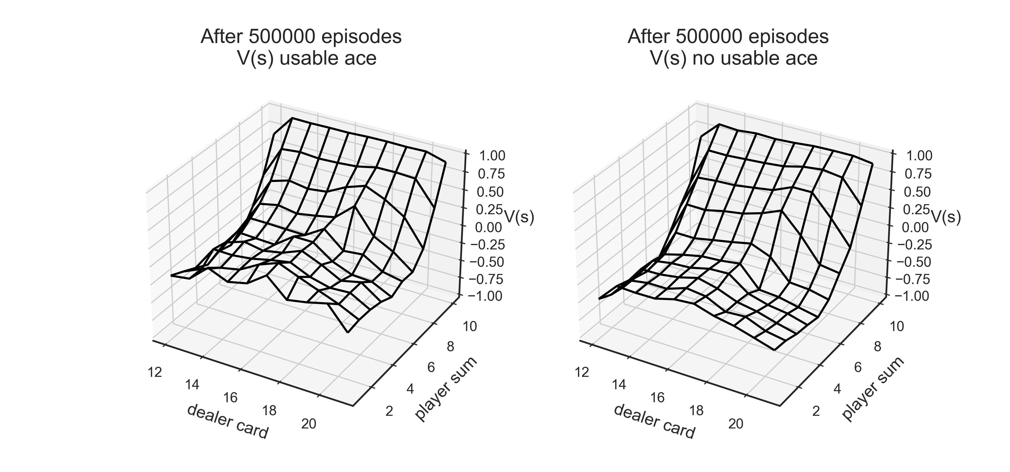
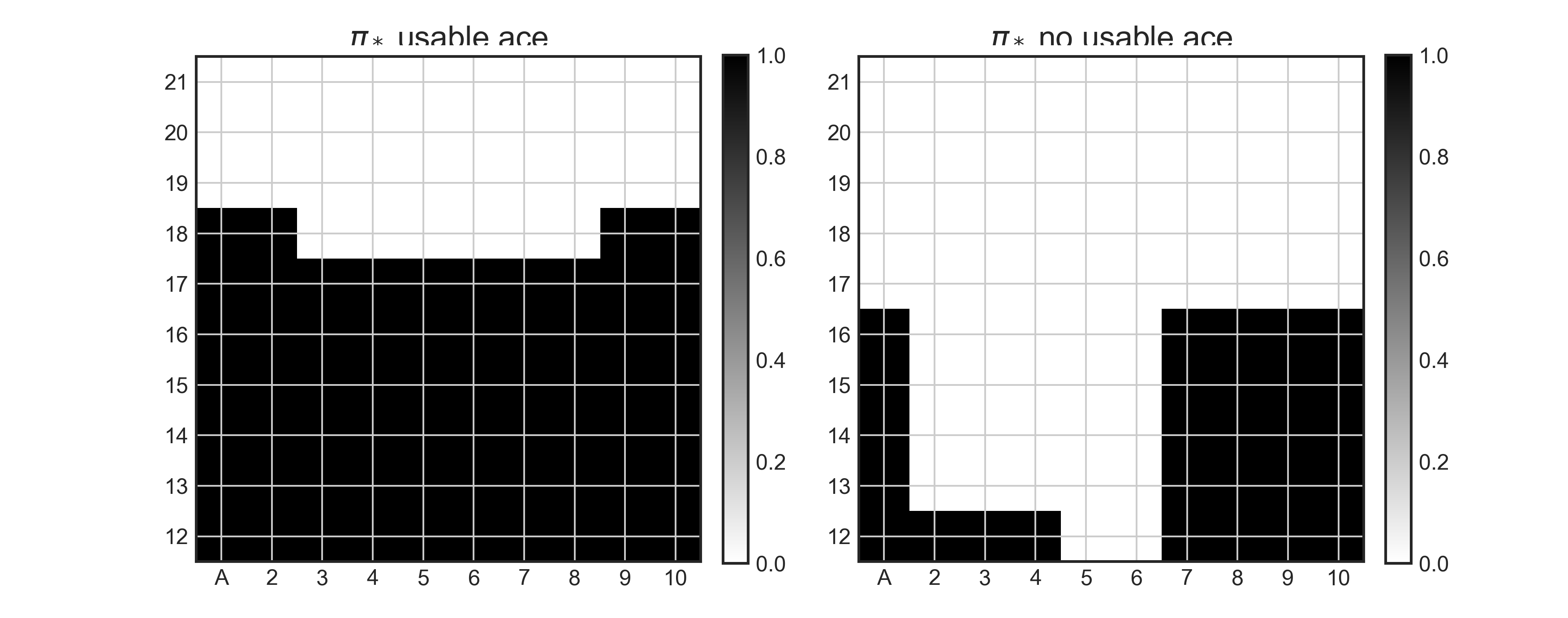
The above corresponds to Figure 5.2: hit-black(1), stick-white(0)
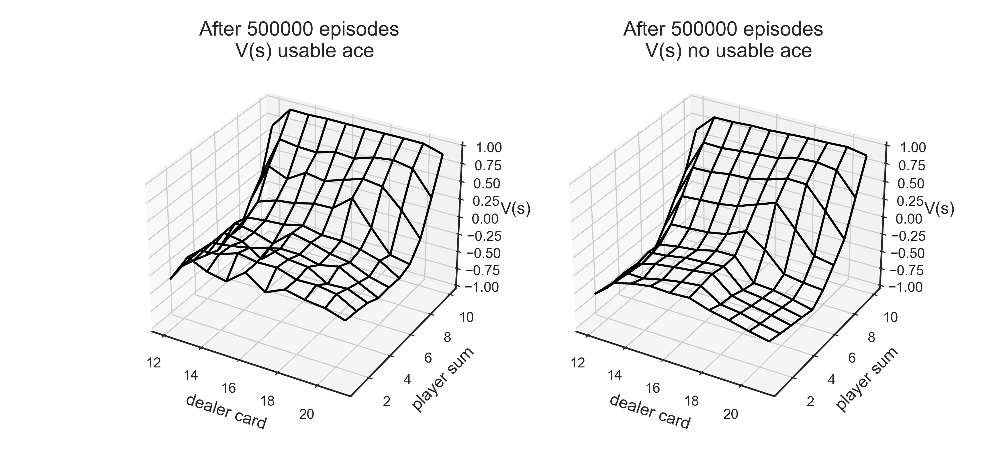
on-policy Monte Carlo
- use epsilon-greedy policy with 95% greedy action and 5% non-greedy random action
def e_greedy(Q,s,epsilon,na):

    prob=np.ones(na, dtype=float)*epsilon/na
    best_a=np.argmax(Q[s])
    prob[best_a]+=1.-epsilon
    #for example there is 95% for taking greedy(best) action, 5% for random action
    #prob=prob[::-1]
    return np.random.choice(np.arange(na),p=prob),prob

def mc_egreedy(env,n_eps,gm=1.0,epsilon=0.1):

    ret_sum=defaultdict(float)
    ret_cnt=defaultdict(float)

    na=env.action_space.n
    Q=defaultdict(lambda: np.zeros(na))

    for ep in range(n_eps):
        traj=[]
        s=env.reset()

        for i in range(100):
            a,prob=e_greedy(Q,s,epsilon,na)
            s_,r,done,_=env.step(a)
            traj.append((s,a,r))

            if done:
                break
            s=s_

        # find the unique state-action pairs
        pairs=set([(t[0], t[1]) for t in traj])

        for (s,a) in pairs:
            pair=(s,a)
            # find the first occurence of each state-action pairs
            idx=traj.index([t for t in traj if t[0]==s and t[1]==a][0])
            V=sum([t[2]*gm**i for i, t in enumerate(traj[idx:])])

            ret_sum[pair]+=V
            ret_cnt[pair]+=1.

            Q[s][a]=ret_sum[pair]/ret_cnt[pair]

    V=defaultdict(float)
    for s, a_s in Q.items():
        V[s]=np.max(a_s)

    return Q,V,policy

Q,V,pi=mc_egreedy(env,500000)

fig,axes=plt.subplots(ncols=2,figsize=(10,10),subplot_kw={'projection': '3d'})

axes[0].set_title('After 500000 episodes \n V(s) usable ace')
axes[1].set_title('After 500000 episodes \n V(s) no usable ace')

plot_blackjack(V,axes[0],axes[1])
off-policy Monte Carlo
for value estimation:
Evaluate the state of [13,2,True]:
    player's card: 13
    dealter's showing: 2
    has usable ace: True

Behavior policy: equally random [hit,stick]=[0.5,0.5]
Target policy: stick only on a sum of 20 and 21

True value of V(13,2,True) is approximately -0.27726

Both Ordinary and Weighted Importance sampling can approximate this value after 1000 off-policy episodes using the random behavior policy
def sample_policy(s):

    player_card, _, _ = s
    return 0 if player_card >= 20 else 1

def behavior_policy(na):

    return np.ones(na,dtype=float)/na

def offpolicy_mc(n_eps):

    sum_ratio=[0]
    sum_ret=[0]
    na=env.action_space.n

    for ep in range(n_eps):
        s=env.reset()
        s=(13,2,True)
        traj=[]

        for i in range(100):
            prob=behavior_policy(na)
            a=np.random.choice(np.arange(na),p=prob)
            s_,r,done,_=env.step(a)
            traj.append((s,a,r))
            if done:
                break
            s=s_

        #numerator and denominator for importance ratio
        nu,de=1.,1.
        for s,a,r in traj:
            if a==sample_policy(s):
                de*=0.5
            else:
                nu=0.
                break

        ratio=nu/de
        sum_ratio.append(sum_ratio[-1]+ratio)
        sum_ret.append(sum_ret[-1]+r*ratio)

    del sum_ratio[0]
    del sum_ret[0]

    sum_ret=np.asarray(sum_ret)
    sum_ratio=np.asarray(sum_ratio)

    ordinary_sampling=sum_ret/np.arange(1,n_eps+1)

    with np.errstate(divide='ignore',invalid='ignore'):
        weighted_sampling=np.where(sum_ratio!=0, sum_ret/sum_ratio,0)

    return ordinary_sampling, weighted_sampling

true_v=-0.27726
n_eps=10000
n_run=100
mse_ord=np.zeros(n_eps)
mse_wei=np.zeros(n_eps)

for i in range(n_run):

    ord,wei=offpolicy_mc(n_eps)
    mse_ord+=np.power(ord-true_v,2)
    mse_wei+=np.power(wei-true_v,2)

mse_ord/=n_run
mse_wei/=n_run

plt.plot(mse_ord,label='Ordinary Importance Sampling',color='g')
plt.plot(mse_wei,label='Weighted Importance Sampling',color='r')
plt.ylim(-0.1, 5)
plt.xscale('log')
plt.legend()
plt.xlabel('Episodes (log scale)')
plt.ylabel('MSE over 100 runs')
#plt.savefig('blackjack_offmc_estimation.png',dpi=350)
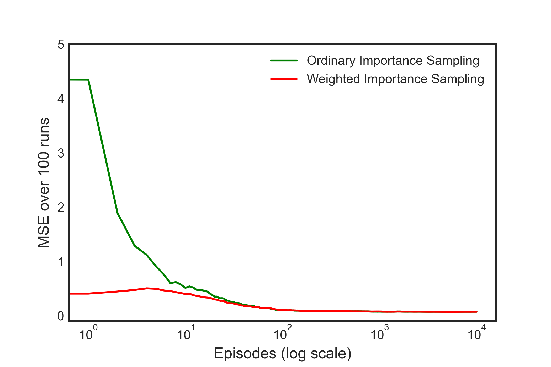
The above corresponds to Figure 5.3, showing Weighted Importance Sampling produces lower error estimates of the value from off-policy episodes
for optimal policy estimation:
def behavior_policy(na):

    return np.ones(na,dtype=float)/na

def target_policy(Q,s,na):

    best_a=np.argmax(Q[s])
    prob=np.zeros(na,dtype=float)
    prob[best_a]=1.

    return prob

def mc_importance_sampling(env,n_eps,gm=1.0):

    na=env.action_space.n
    #numerator and denumerator for importance sampling ratio
    nu=defaultdict(lambda: np.zeros(na))
    de=defaultdict(lambda: np.zeros(na))
    Q=defaultdict(lambda: np.zeros(na))

    for ep in range(n_eps):
        s=env.reset()
        traj=[]

        for i in range(100):
            prob=behavior_policy(na)
            a=np.random.choice(np.arange(na), p=prob)
            s_,r,done,_=env.step(a)
            traj.append((s,a,r))
            if done:
                break
            s=s_

        #find unique state-aciton pairs
        pairs=set([(t[0], t[1]) for t in traj])

        for (s,a) in pairs:
            pair=(s,a)

            # find the first occurence of this pair in traj
            # t[0]-s, t[1]-a, t[2]-r
            idx=traj.index([t for t in traj if t[0]==s and t[1]==a][0])

            V=sum([t[2]*gm**i for i,t in enumerate(traj[idx:])])

            #calculate product of 1./b(a|s) of each state-action pair
            w=np.product([1./behavior_policy(na)[t[1]] for t in traj[idx:]])

            nu[s][a]+=w*V
            de[s][a]+=w

            Q[s][a]=nu[s][a]/de[s][a]

    return Q

Q=mc_importance_sampling(env,n_eps=500000)

V=defaultdict(float)
for s, a_v in Q.items():
    V[s]=np.max(a_v)

fig,axes=plt.subplots(ncols=2,figsize=(10,10),subplot_kw={'projection': '3d'})

axes[0].set_title('After 500000 episodes \n V(s) usable ace')
axes[1].set_title('After 500000 episodes \n V(s) no usable ace')

plot_blackjack(V,axes[0],axes[1])
#plt.savefig('blackjack_offmc_importance_sampling.png',dpi=350)
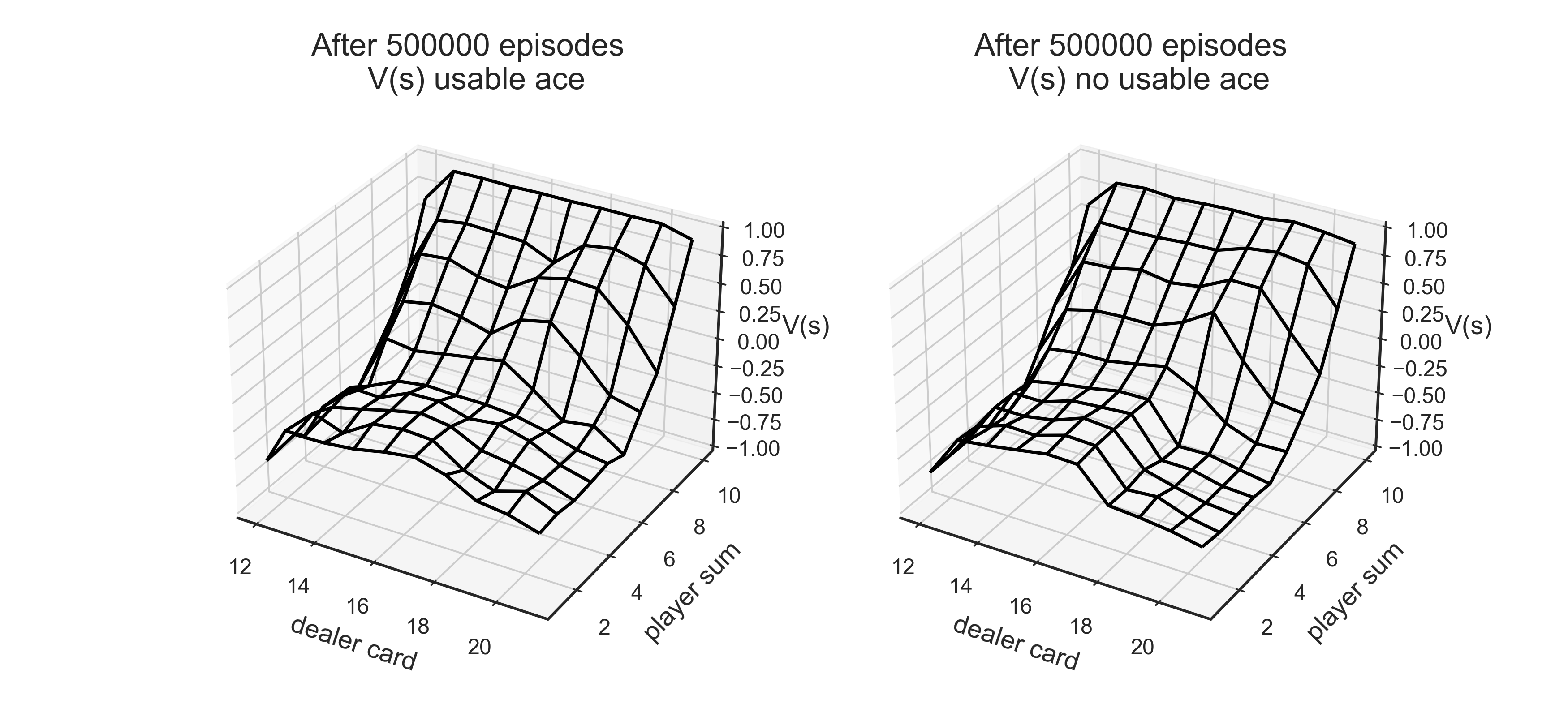
Target policy can be inferred from the obtained Q value in terms of certain states
References
Reinforcement Learning an Introduction 2nd edition, Chapter 3,4,5 by Sutton and Barto
RL simple experiment - Blackjack
optimizing blackjack strategy through MC
ShangtongZhang/reinforcement-learning-an-introduction
jingweiz/reinforcement-learning-an-introduction
RL 2nd Edition Excercise Solutions