Bias and Variance
Expectation
Def: the weighted average of a function \(f(x)\) weighted by a probability distribution \(p(x)\) that generates data
For a discrete distribution:
\[\mathbb{E}_{x \sim p(x)}[f(x)]=\sum_x p(x)f(x)\]In the case of continuous variables with their probability densities:
\[\mathbb{E}_{x \sim p(x)}[f(x)]=\int p(x)f(x) dx\]In either case, if we are given a finite number \(N\) of points drawn from the probability distribution or probability density, the expectation can be approximated as a finite sum over these points
\[\mathbb{E}[f(x)] \simeq \frac{1}{N} \sum_{i=1}^N f(x_i)\]Variance
Def: a measure of how much variability there is in \(f(x)\) around its mean \(\mathbb{E}[f(x)]\)
\[var[f(x)]=\mathbb{E}[(f(x)-\mathbb{E}[f(x)])^2]\]If we expand the above
\[\begin{align*} var[f(x)] &= \mathbb{E} [(f(x)-\mathbb{E}[f(x)])^2 ] \\ &= \mathbb{E}[f^2(x)+\mathbb{E}^2[f(x)]-2f(x)\mathbb{E}[f(x)]] \\ &= \mathbb{E}[f^2(x)]+\mathbb{E}^2[f(x)]-2\mathbb{E}^2[f(x)] \\ &= \mathbb{E}[f^2(x)]-\mathbb{E}^2[f(x)] \end{align*}\]We will have the variance with two expectations of \(f(x)\) and \(f^2(x)\)
We may also consider the variance of a variable \(x\) itself:
\[\begin{align*} var[x] &=\mathbb{E}[(x-\mathbb{E}[x])^2] \\ &=\mathbb{E}[x^2]-\mathbb{E}^2[x] \end{align*}\]Bias
Def: the difference of the average value of prediction \(\hat{f}(x)\) from the true function \(f(x)\)
\[bias[\hat{f}(x)]=\mathbb{E}[\hat{f}(x)]-f(x)\]If a prediction is unbiased
\[\mathbb{E}[\hat{f}(x)]=f(x)\]Naive sample variance is biased
Suppose we have a sample mean
\[\hat{\mu}=\frac{1}{N} \sum_i^N x_i\]and a naive sample variance, which can be derived from Maximum Likelihood method in the case of Gaussian distribution
\[\hat{\sigma}^2=\frac{1}{N} \sum_i^N (x_i-\hat{\mu})^2\]\(\hat{\sigma}^2\) is a biased estimator because
\[\begin{align*} \mathbb{E}[\hat{\sigma}^2] &= \mathbb{E} \left[\frac{1}{N} \sum_i^N (x_i-\hat{\mu})^2 \right] \\ &= \mathbb{E} \left[\frac{1}{N} \sum \left((x_i-\mu)-(\hat{\mu}-\mu) \right)^2 \right] \\ &= \mathbb{E} \left[\frac{1}{N} \sum \left((x_i-\mu)^2-2(\hat{\mu}-\mu)(x_i-\mu) +(\hat{\mu}-\mu)^2 \right) \right] \\ &= \mathbb{E} \left[\frac{1}{N} \sum (x_i-\mu)^2-\frac{2}{N}(\hat{\mu}-\mu)\sum (x_i-\mu) +\frac{1}{N} (\hat{\mu}-\mu)^2 \sum 1 \right] \\ &= \mathbb{E} \left[\frac{1}{N} \sum (x_i-\mu)^2-\frac{2}{N}(\hat{\mu}-\mu)\sum (x_i-\mu) + \frac{1}{N} (\hat{\mu}-\mu)^2 \cdot N \right] \\ &= \mathbb{E} \left[\frac{1}{N} \sum (x_i-\mu)^2-\frac{2}{N}(\hat{\mu}-\mu)\underbrace{\sum(x_i-\mu)}_{=N(\hat{\mu}-\mu), (*1)} + (\hat{\mu}-\mu)^2 \right] \\ &= \mathbb{E}\left[\frac{1}{N} \sum (x_i-\mu)^2- (\hat{\mu}-\mu)^2 \right] \\ &= \mathbb{E}\left[\frac{1}{N} \sum (x_i-\mu)^2\right] - \mathbb{E}\left[ (\hat{\mu}-\mu)^2 \right] \\ &= \underbrace{\frac{1}{N} \sum \mathbb{E}\left[(x_i-\mu)^2\right]}_{=\sigma^2, (*2)} - \underbrace{\mathbb{E}\left[ (\hat{\mu}-\mu)^2 \right]}_{=\frac{1}{N}\sigma^2, (*3)} \\ &=\sigma^2-\frac{\sigma^2}{N} \\ &=\frac{N-1}{N} \sigma^2 \end{align*}\]Note \((*1)\):
\[\begin{align*} \hat{\mu}-\mu &=(\frac{1}{N}\sum x_i) - \mu \\ &= (\frac{1}{N}\sum x_i) - (\frac{1}{N}\sum \mu) \\ &= \frac{1}{N}\sum (x_i - \mu) \\ N\cdot(\hat{\mu}-\mu) &= \sum (x_i - \mu) \end{align*}\]\((*2)\):
\[\mathbb{E}\left[(x_i-\mu)^2\right]=var[x_i]=\sigma^2\] \[\frac{1}{N} \sum \mathbb{E}\left[(x_i-\mu)^2\right]=\frac{1}{N} \cdot N \sigma^2=\sigma^2\]\((*3)\):
\[\begin{align*} \mathbb{E}\left[ (\hat{\mu}-\mu)^2 \right] &=var[\hat{\mu}] \\ &=var \left[\frac{x_1+x_2+...x_N}{N} \right] \\ &=var \left[\frac{x_1}{N}+\frac{x_2}{N} + ... \right] \\ &= \frac{1}{N^2}var[x_1]+ \frac{1}{N^2}var[x_2]+... (*4)\\ &= \frac{1}{N^2} [\sigma^2+\sigma^2+...] \\ &=\frac{1}{N^2} \cdot N\sigma^2 \\ &=\frac{\sigma^2}{N} \end{align*}\]\((*4)\):
we can easily derive \(var[cx]=c^2 var[x]\), where \(c\) is a scalar
Recall
\[\mathbb{E}[\hat{\mu}]=\frac{1}{N} \sum \mathbb{E}[x_i]=\mu\]so \(\hat{\mu}\) is an unbiased estimator of \(\mu\)
However
\[\mathbb{E}[\hat{\sigma}^2]= \frac{N-1}{N} \sigma^2 \neq \sigma^2\]so \(\hat{\sigma}^2\) is a biased estimator of \(\sigma^2\)
To obtain an unbiased estimator of \(\sigma\), we need a correction
\[\tilde{\sigma}^2=\frac{N}{N-1}\hat{\sigma}^2=\frac{1}{N-1} \sum (x_i-\hat{\mu})^2\]For another way of proof, see the exercise solution of PRML 1.12
Example
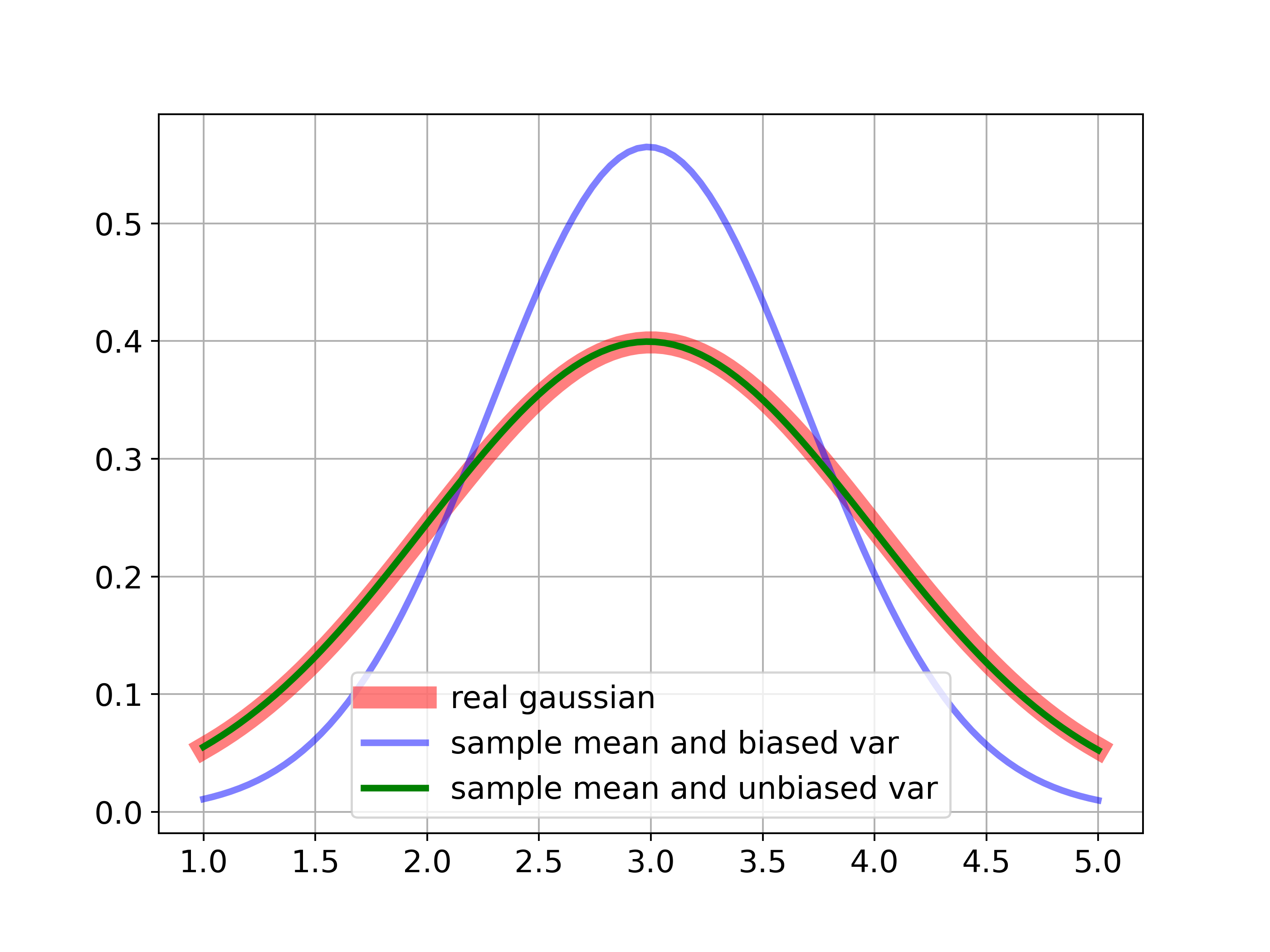
Let’s generate 10000 datasets with only 2 data points for each from \(\mathcal{N}(3,1)\)
We use this 2 data points for estimating sample mean and (biased and unbiased) variance and take average across 10000 datasets to see their performances
import numpy as np
import matplotlib.pyplot as plt
plt.rcParams['font.size']='14'

np.random.seed(3)
#real
x=np.linspace(1,5,num=100)

def gaussian(x,mu,sig2):
    return np.exp(((x-mu)**2)/(-2*sig2))/np.sqrt(2*np.pi*sig2)

mu,sig2=3,1.

#generate 10000 data sets with only two data
N=2 #number of data in each dataset
M=10000 #number of dataset
samples=np.sqrt(sig2)*np.random.randn(N,M)+mu

#sample mean
mu_hat=(1./N)*samples.sum(0)
#biased sample var
sig2_hat=(1./N)*((samples-mu_hat)**2).sum(0)
#unbiased sample var
sig2_hat_unbiased=(1./(N-1))*((samples-mu_hat)**2).sum(0)

plt.figure(figsize=(8,6))
plt.plot(x,gaussian(x,mu,sig2),'r',linewidth=10,label='real gaussian',alpha=.5)
plt.plot(x,gaussian(x,mu_hat.sum(0)/M,sig2_hat.sum(0)/M),'b',linewidth=3,label='sample mean and biased var', alpha=0.5)
plt.plot(x,gaussian(x,mu_hat.sum(0)/M,sig2_hat_unbiased.sum(0)/M),'g',linewidth=3,label='sample mean and unbiased var')

plt.grid()
plt.legend()
plt.savefig('un_bias_variance.png',dpi=350)

This experiment shows the difference between biased sample variance (blue) and unbiased sample variance (green). The latter has a good fit with the true distribution
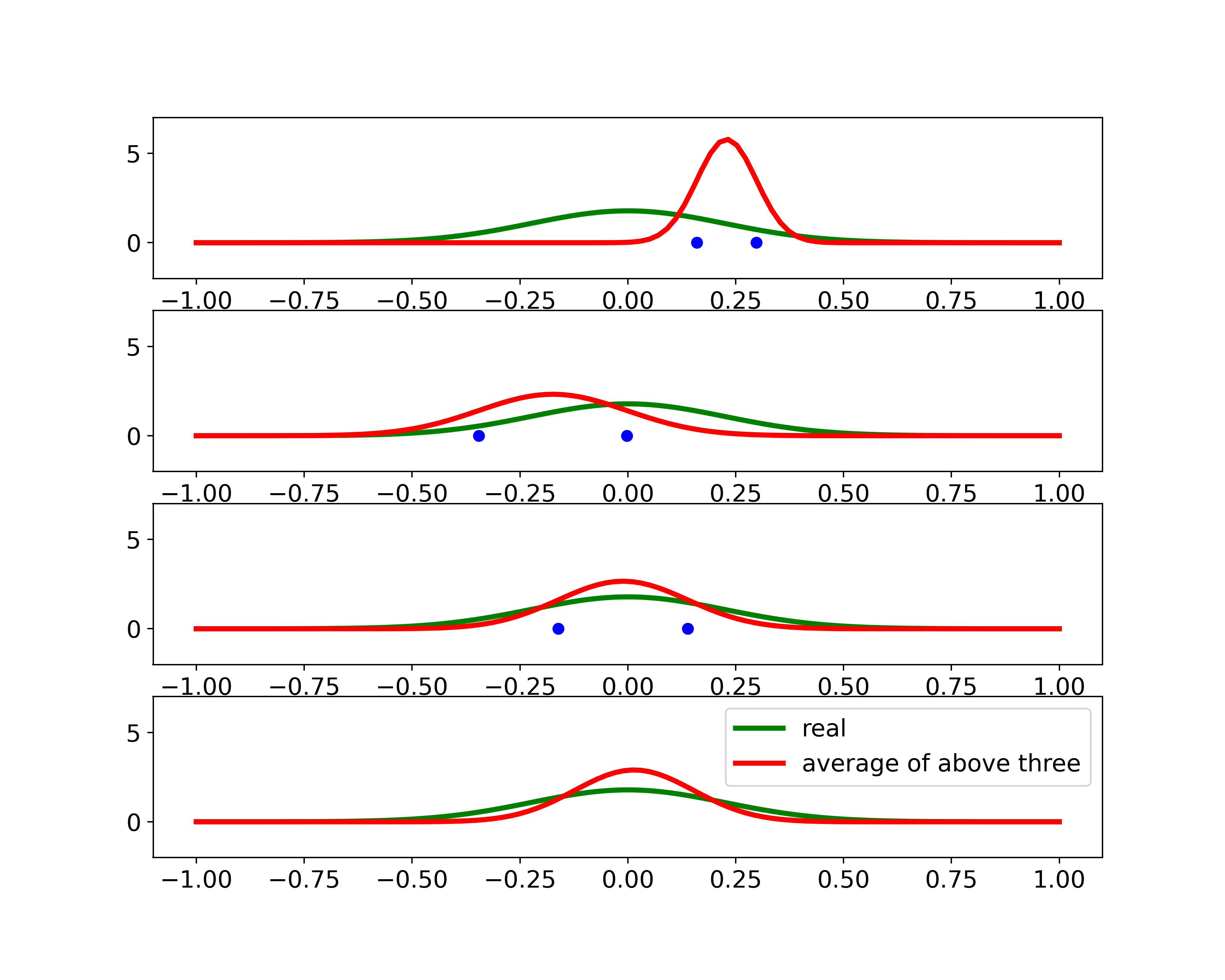
We use another Gaussian example to show why the bias arises
np.random.seed(10)

x=np.linspace(-1,1,100)
mu,sig2=0,0.05
N=2 #sample size

plt.figure(figsize=(10,8))
for i in range(3):
    plt.subplot(3,1,i+1)
    plt.ylim([-2,7])

    sample=np.random.randn(N)*np.sqrt(sig2)+mu
    plt.plot(sample,[0,0],'bo')

    mu_hat=sample.sum()/N
    sig2_hat=((sample-mu_hat)**2).sum()/N

    plt.plot(x,gaussian(x,mu,sig2),'g',linewidth=3,label='real')
    plt.plot(x,gaussian(x,mu_hat,sig2_hat),'r',linewidth=3,label='sample mean and var')

plt.legend()
plt.savefig('3_bias_variance.png',dpi=350)

The above corresponds to Figure 1.15 in PRML
This experiment indicates that with 3 small datasets each with 2 samples, the unbiased mean can be captured, as the red curve shown in the fourth row. However, the variance is under-estimated because it is measured relative to the sample mean and not relative to the true mean
This issue will be less significant as the number of samples increases
Bias and Variance in model fitting
Bias: the inability of a model to accurately capture the true pattern of data
\[bias[\hat{f}(x)]=\mathbb{E}[\hat{f}(x)]-f(x)\]for example, if we use a line to fit a quadratic model, the bias is high
Variance: the amount by which the estimate of the true pattern would change on using a different dataset
\[var[\hat{f}(x)]=\mathbb{E}[(\hat{f}(x)-\mathbb{E}[\hat{f}(x)])^2]\]for example, high variance implies that the model does not generalize well on unseen data even if it fits the training data well
Overfitting: low bias and high variance, model fits the training data well, but captures noise
Underfitting: high bias and low variance, model fails to capture the pattern of the data at all
Bias-Variance Trade-off
Def: a way to ensure that the model is neither overfitted nor underfitted
Ideally, a model should have low bias and low variance
Suppose our data is generated in this form:
\[y=f(x)+\epsilon\]where
\((x,y)\) <- data
\(f(x)\) <- the true relationship of data (hard to know in real life)
\(\epsilon\) <- the irreducible noise with zero mean and variance \(\sigma_{\epsilon}^2\)
Now we try to model the true pattern of \(f(x)\) by a function \(\hat{f}(x)\)
The goal is to bring the prediction \(\hat{f}(x)\) as close as possible to the actual value \(y\): \(\hat{f}(x) \rightarrow y\) to minimize the error
Here comes the bias-variance trade-off equation:
\[\mathbb{E}[(y-\hat{f}(x))^2]=bias[\hat{f}(x)]^2+var[\hat{f}(x)]+\sigma_{\epsilon}^2\]where
\(\mathbb{E}[(y-\hat{f}(x))^2]\) <- Mean Squared Error (MSE)
\(bias[\hat{f}(x)]=\mathbb{E}[\hat{f}(x)]-f(x)\) <- Bias
\(var[\hat{f}(x)]=\mathbb{E}[(\hat{f}(x)-\mathbb{E}[\hat{f}(x)])^2]\) <- Variance
Proof:
\[\begin{align*} \mathbb{E}[(y-\hat{f}(x))^2] &= \mathbb{E}[(f(x)+\epsilon-\hat{f}(x))^2] \\ &= \mathbb{E}[(f(x)-\hat{f}(x))^2]+\mathbb{E}[\epsilon^2]+2\mathbb{E}[(f(x)-\hat{f}(x))\epsilon] \\ &= \mathbb{E}[(f(x)-\hat{f}(x))^2]+\underbrace{\mathbb{E}[\epsilon^2]}_{=\sigma_{\epsilon}^2}+2\mathbb{E}[(f(x)-\hat{f}(x))]\underbrace{\mathbb{E}[\epsilon]}_{=0} \\ &= \mathbb{E}[(f(x)-\hat{f}(x))^2]+\sigma_{\epsilon}^2 \\ &= \mathbb{E}\left[((f(x)-\mathbb{E}[\hat{f}(x)])-(\hat{f}(x)-\mathbb{E}[\hat{f}(x)]))^2 \right] +\sigma_{\epsilon}^2 \\ &= \mathbb{E}\left[(f(x)-\mathbb{E}[\hat{f}(x)])^2+(\hat{f}(x)-\mathbb{E}[\hat{f}(x)])^2-2(f(x)-\mathbb{E}[\hat{f}(x)])(\hat{f}(x)-\mathbb{E}[\hat{f}(x)]) \right] +\sigma_{\epsilon}^2 \\ &= \mathbb{E}\left[(f(x)-\mathbb{E}[\hat{f}(x)])^2 \right]+\mathbb{E}\left[(\hat{f}(x)-\mathbb{E}[\hat{f}(x)])^2 \right]-2\mathbb{E}\left[(f(x)-\mathbb{E}[\hat{f}(x)])(\hat{f}(x)-\mathbb{E}[\hat{f}(x)]) \right] +\sigma_{\epsilon}^2 \\ &= [\underbrace{f(x)-\mathbb{E}[\hat{f}(x)]}_{=bias[\hat{f}(x)],(*5)}]^2 +\underbrace{\mathbb{E}\left[(\hat{f}(x)-\mathbb{E}[\hat{f}(x)])^2 \right]}_{=var[\hat{f}(x)]}-2\underbrace{(f(x)-\mathbb{E}[\hat{f}(x)])}_{\text{constant}} \underbrace{\mathbb{E}\left[(\hat{f}(x)-\mathbb{E}[\hat{f}(x)]) \right]}_{=\mathbb{E}[\hat{f}(x)]-\mathbb{E}[\hat{f}(x)]=0} +\sigma_{\epsilon}^2 \\ &= bias[\hat{f}(x)]^2+var[\hat{f}(x)]+\sigma_{\epsilon}^2 \end{align*}\]\((*5)\):
since \(f(x)-\mathbb{E}[\hat{f}(x)]\) is a constant minus a constant
\[\mathbb{E}[(f(x)-\mathbb{E}[\hat{f}(x)])^2]=(f(x)-\mathbb{E}[\hat{f}(x)])^2\]Example
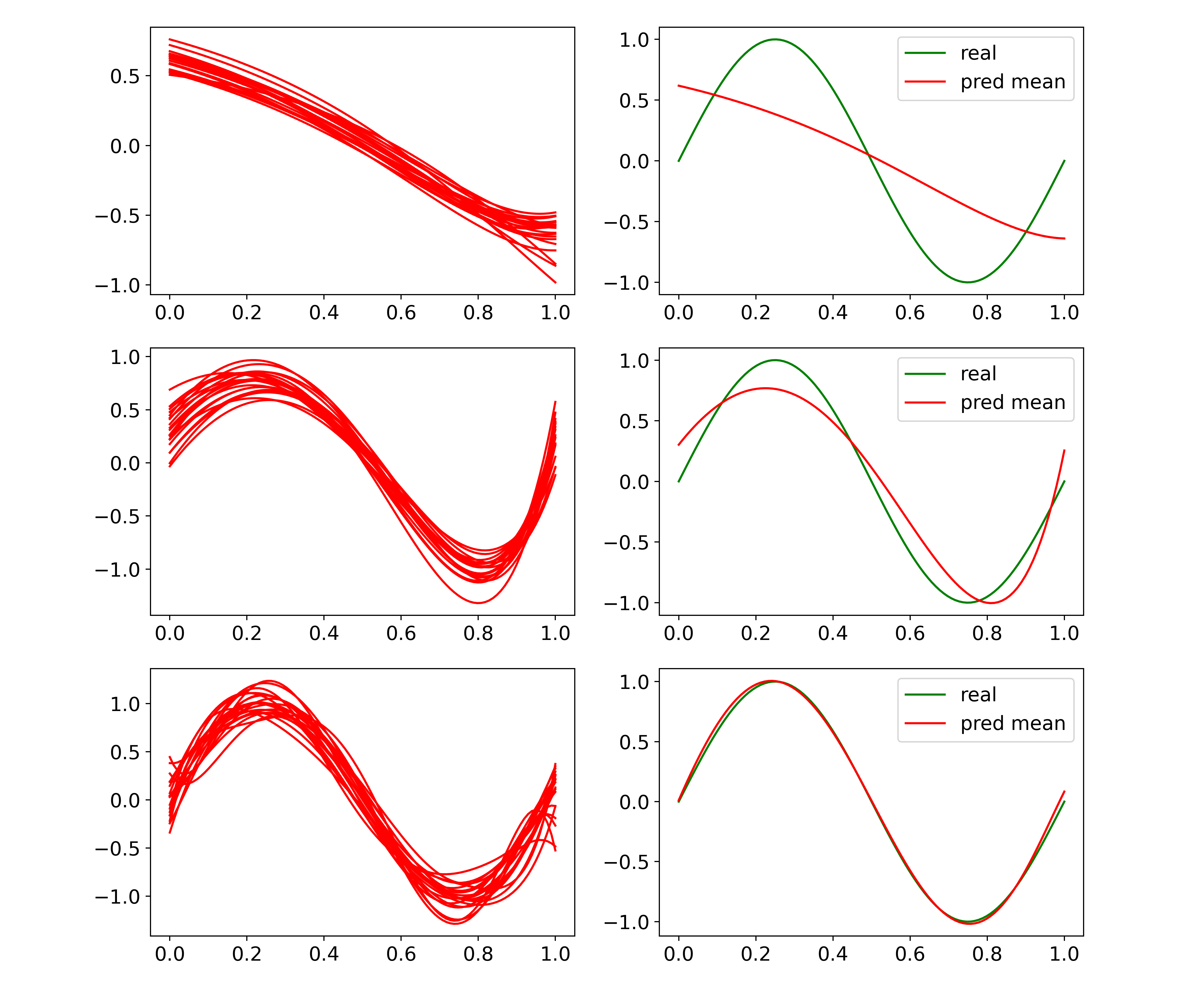
We show an example from Ridge Regression by altering different \(\lambda\) parameters for the regularizer term
Note Ridge Regression has the l2 norm of the regularizer in the objective function
\[obj = ||y-\hat{f}(\textbf{x})||^2+\lambda ||\textbf{w}||^2_2\]where \(\hat{f}(\textbf{x})=\textbf{wx}\)
We use Polynomial Features from sklearn for the basis functions (a bit different from the PRML figure 3.5), and bias_variance_decomp from mlxtend for decomposing bias and variance from the objective error
from sklearn.preprocessing import PolynomialFeatures
from sklearn.linear_model import Ridge

np.random.seed(5)

lmd_smooth=[1,0.1,0.01,0.005,0.001,0.0001,0.000001,0.0000001,0.000000001]
label=[0,3,8]
lmd_all=[lmd_smooth[i] for i in label]
#test/real
x=np.linspace(0,1,100)
y=np.sin(2*np.pi*x)

plt.figure(figsize=(12,12))
for n,lmd in enumerate(lmd_all):
    f_pred_all=[]
    for i in range(20):
        #training data
        x_25=np.linspace(0,1,25) #sample size=25
        y_25=np.sin(2*np.pi*x_25)+np.random.normal(scale=0.25,size=x_25.shape)

        #polytransformed
        f=PolynomialFeatures(degree=6).fit_transform(x.reshape(-1,1))
        f_25=PolynomialFeatures(degree=6).fit_transform(x_25.reshape(-1,1))

        ridge=Ridge(lmd)
        ridge.fit(f_25,y_25)

        f_pred=ridge.predict(f)
        f_pred_all.append(f_pred)
        plt.subplot(3,2,2*n+1)
        plt.plot(x,f_pred,'r',label='pred')

    plt.subplot(3,2,2*n+2)
    plt.plot(x,y,'g',label='real')
    plt.plot(x,np.array(f_pred_all).mean(0),'r',label='pred mean')
    plt.legend()

plt.savefig('ridge_bias_variance.png',dpi=350)

The above corresponds to Figure 3.5 in PRML
This experiment shows that different \(\lambda\) indicates different model complexity
Larger \(\lambda\) like figure in the first row suggests higher bias, and lower variance, while lower \(\lambda\) like figure in the third row suggests lower bias, and higher variance
from mlxtend.evaluate import bias_variance_decomp
lmd_smooth=[1,0.1,0.01,0.005,0.001,0.0001,0.000001,0.0000001,0.000000001]
err_all,bias_all,var_all=[],[],[]
for lmd in lmd_smooth:
    error,bias,var=bias_variance_decomp(Ridge(lmd),f_25,y_25,f,y,loss='mse',random_seed=5)
    err_all.append(error)
    bias_all.append(bias)
    var_all.append(var)

plt.figure(figsize=(8,6))
plt.plot(err_all,'-o',markersize=10,linewidth=3,label='error')
plt.plot(bias_all,'-o',markersize=10,linewidth=3,label='bias')
plt.plot(var_all,'-o',markersize=10,linewidth=3,label='var')
plt.legend()
plt.grid()
plt.xlabel('$\lambda$')
plt.xticks(np.arange(9),[str(lmd) for lmd in lmd_smooth])
plt.savefig('decomp_bias_variance.png',dpi=350)

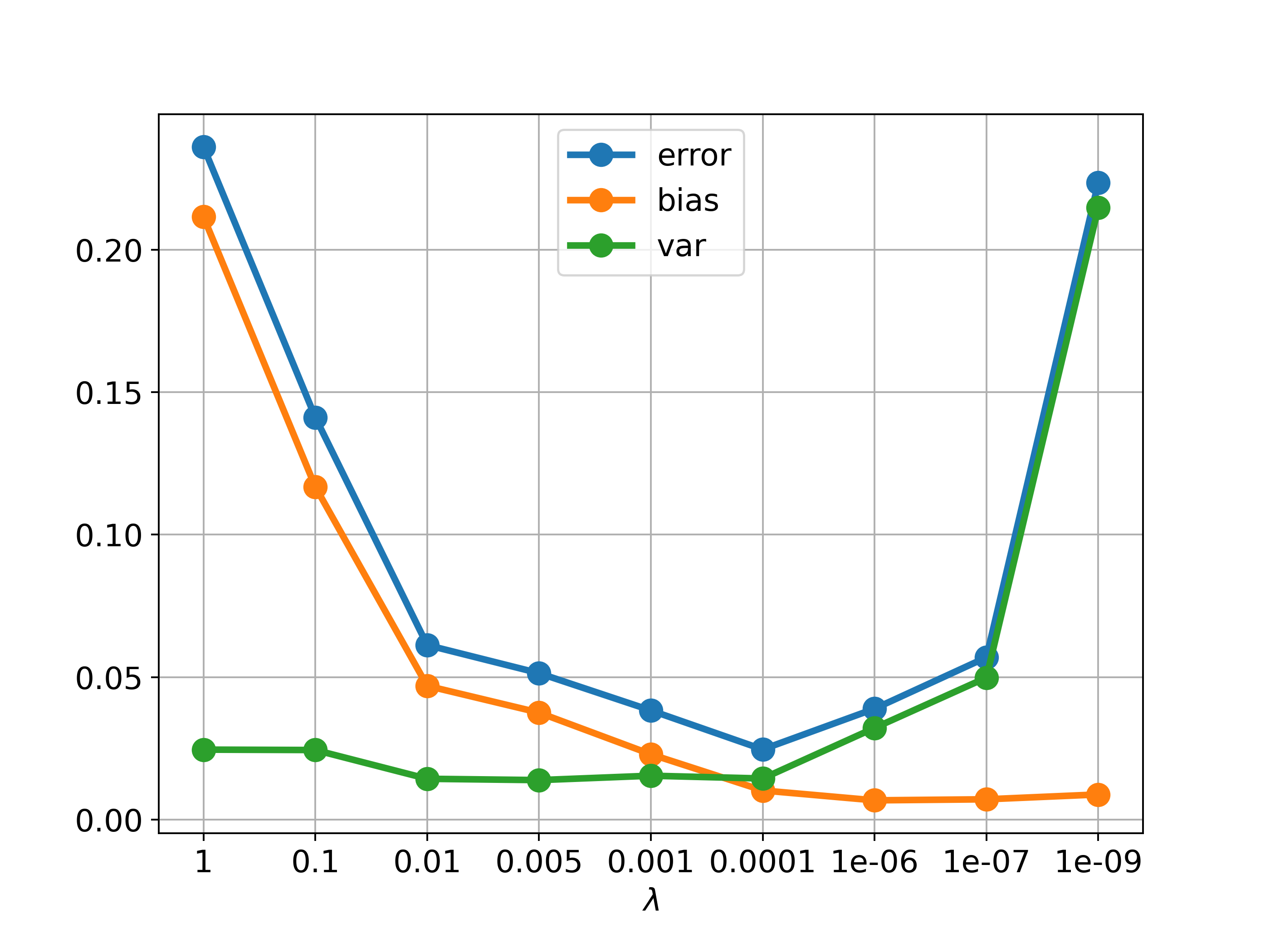
The above corresponds to Figure 3.6 in PRML
This experiment gives a clear picture of how the bias-variance trade-off occurs
An appropriate \(\lambda\) would be 0.0001, which provides the lowest error
References
Pattern Recognition and Machine Learning by Christopher Bishop
Mean and Variance of Sample Mean
PRMLの図作成 図1.15 ガウス分布の最尤推定におけるバイアス
The Bias-Variance Trade-off a mathematical view
【Python】3.1.0:基底関数の作図【PRMLのノート】