Policy Gradient and Actor-Critic

Despite value-based methods where policies were derived from the action-value functions, we can learn a parameterized policy \(\pi(a \mid s, \boldsymbol{\theta})\) directly, with \(\boldsymbol{\theta}\) being the policy parameters

The parameters are updated in a gradient ascent fashion based on a scalar performance measure \(J(\boldsymbol{\theta})\):

\[\boldsymbol{\theta}_{t+1} \leftarrow \boldsymbol{\theta}_t+\alpha \hat{\nabla J(\boldsymbol{\theta}_t)}\]

where \(\hat{\nabla J(\boldsymbol{\theta}_t)} \in \mathbb{R}^d\) is a stochastic estimate whose expectation approximates the gradient of \(J(\boldsymbol{\theta})\)

Advantages of Policy-based Methods

learn a stochastic policy that provides specific probabilities for taking the actions (hard for value-based methods)
this stochasticity could start from appropriate levels of exploration to deterministic policies asymptotically (other than \(\epsilon\)-greedy in valued-based methods)
naturally handle continuous action spaces (hard for value-based methods)
policy may be a simpler function to approximate, so that it learns faster and yields a superior asymptotic policy (this varies in the complexity of the policies and action-value functions)
the choice of policy parameterization is a good way of injecting prior knowledge
the continuity of the policy dependence on the parameters enables the action probabilities to change smoothly and therefore allows for convergence guarantees with gradient ascent
etc

Action Formulations

In order to construct a differentiable policy for discrete action spaces, we often form a softmax policy:

\[\pi(a\mid s, \boldsymbol{\theta}) \triangleq \frac{\exp \boldsymbol{\theta}^T \phi(s,a)}{\sum_b \exp \boldsymbol{\theta}^T \phi(s,b)}\]

where \(\boldsymbol{\theta}^T \phi(s,a)\) is a linear combination of features \(\phi(s,a)\), which can be defined by a parameterized numerical preference \(h(s,a; \boldsymbol{\theta})\)

This suggests that the actions with the highest preferences in each state are given the highest probabilities of being selected

some insights:

this action preference can be defined arbitrarily, i.e. linearly or like neural networks
it is different from action-values, since the latter would converge to their corresponding true values, leading the policy to some specific probabilities other than 0 and 1
the approximate policy by action preference can approach a deterministic policy, since the formulation is driven to produce the optimal stochastic policy (which can also be a deterministic policy)
action preference enables the selection of actions with arbitrary probabilities, where action-value based methods have no natural way of finding stochastic optimal policies

See Short Corridor for more info

In the case of continuous action spaces, we often use Gaussian policy, where the mean is the linear combination of state features:

\[\pi(a\mid s, \boldsymbol{\theta}) \triangleq \mathcal{N}(\boldsymbol{\theta}^T \phi(s), \sigma^2)\]

Policy Gradient Theorem

With the definition of the performance measure being the value of the start state of an episode by assuming that every episode starts in some particular state \(s_0\):

\[J(\boldsymbol{\theta}) \triangleq V_{\pi_{\boldsymbol{\theta}}} (s_0)\]

the Policy Gradient Theorem provides a general link between \(\nabla J(\boldsymbol{\theta})\) and the gradient of the policy \(\nabla \pi(a \mid s)\) itself without taking derivatives of the state distribution:

\[\nabla J(\boldsymbol{\theta}) \propto \sum_{s \in \mathcal{S}} \mu(s) \sum_{a \in \mathcal{A}} Q_{\pi}(s,a) \nabla \pi(a \mid s, \boldsymbol{\theta})\]

See this post for a detailed proof

Here, \(\mu(s)\) is the on-policy distribution under \(\pi\)

Assuming we have far more states than weights, we have to emphasize which states are of more importance by specifying a state distribution:

\[\mu(s) \geq 0, \sum_{s \in \mathcal{S}} \mu(s)=1\]

Under on-policy training this is called on-policy distribution, and often \(\mu(s)\) is chosen to be the fraction of time spent in \(s\)

In continuous tasks, it is the stationary distribution under a specific policy defined by \(d^\pi (s)\):

\[d^\pi (s) \triangleq \lim_{t \rightarrow \infty} P(s_t=s \mid s_0, \pi_{\boldsymbol{\theta}})\]

where \(P(s_t=s \mid s_0, \pi_{\boldsymbol{\theta}})\) represents the probability of arriving at the state \(s_t\) from \(s_0\) following \(\pi_{\boldsymbol{\theta}}\) in \(t\) steps

It means, when you travel along a Markov Chain in an infinite scale by following one certain policy, the final probability of visiting one state will be unchanged

REINFORCE

The right-hand side of the policy gradient theorem is a sum over states weighted by how often the states occur under the target policy \(\pi\). If \(\pi\) is followed, then states will be encountered in these proportions. Thus, we can write

\[\begin{align*} \nabla J(\boldsymbol{\theta}) &\propto \sum_{s \in \mathcal{S}} \mu(s) \sum_{a \in \mathcal{A}} Q_{\pi}(s,a) \nabla \pi(a \mid s, \boldsymbol{\theta}) \\ &= \mathbb{E}_{\pi} \left[\sum_a Q_{\pi}(s_t,a) \nabla \pi(a \mid s_t, \boldsymbol{\theta}) \right] \end{align*}\]

where \(s_t\) represents the state sample at time \(t\). We can do the same sampling trick to the action \(a_t\), where an appropriate sum over actions like \(\sum_a \pi(a \mid s_t, \boldsymbol{\theta})\) can be replaced by an expectation under \(\pi\). Following the above equations

\[\begin{align*} \nabla J(\boldsymbol{\theta}) &= \mathbb{E}_{\pi} \left[\sum_a \pi(a \mid s_t, \boldsymbol{\theta}) Q_{\pi}(s_t,a) \frac{\nabla \pi(a \mid s_t, \boldsymbol{\theta})}{\pi(a \mid s_t, \boldsymbol{\theta})} \right] \\ &= \mathbb{E}_{\pi} \left[Q_{\pi}(s_t,a_t) \frac{\nabla \pi(a_t \mid s_t, \boldsymbol{\theta})}{\pi(a_t \mid s_t, \boldsymbol{\theta})} \right] \\ &= \mathbb{E}_{\pi} \left[R_t \frac{\nabla \pi(a_t \mid s_t, \boldsymbol{\theta})}{\pi(a_t \mid s_t, \boldsymbol{\theta})} \right] \\ &= \mathbb{E}_{\pi} \left[R_t \nabla \log \pi(a_t \mid s_t, \boldsymbol{\theta}) \right] \end{align*}\]

Since the fraction of \(\frac{\nabla \pi(a_t \mid s_t, \boldsymbol{\theta})}{\pi(a_t \mid s_t, \boldsymbol{\theta})}\) can be replaced with \(\nabla \log \pi(a_t \mid s_t, \boldsymbol{\theta})\), the so-called eligibility vector by applying log-likelihood trick based on the derivative law \(\nabla \log x = \frac{\nabla x}{x}\)

Note that \(R_t\) is the discounted sum of reward starting from time step \(t\):

\[R_t \triangleq \sum_{i=0}^T \gamma^i r_{t+i}\]

and \(Q_{\pi}(s_t, a_t)\) is the expected return starting from \(s_t, a_t\) following \(\pi\):

\[Q_{\pi}(s_t, a_t) \triangleq \mathbb{E}_{\pi} \left[R_t \mid s_t, a_t \right]\]

Therefore, we obtained a quantity that can be sampled on each time step whose expectation is equal to the gradient

The update rule of REINFORCE:

\[\boldsymbol{\theta}_{t+1} \leftarrow \boldsymbol{\theta}_t+\alpha R_t \nabla \log \pi(a_t \mid s_t, \boldsymbol{\theta}_t)\]

See this post for a more intuitive explanation

REINFORCE uses \(R_t\), the complete return from time \(t\) , which includes all future rewards up until the end of the episode, so it is a Monte Carlo method

Summary of REINFORCE:

(+) a stochastic policy/gradient method

(+) theoretical convergence properties

(+) the expected updated is in the same direction as the performance gradient, therefore, it assures an improvement in expected performance for sufficiently small learning rate, and convergence to a local optima

(-) of high variance as a Monte Carlo method, slow learning

(-) policy has to be differentiable

REINFORCE with baseline

One technique to reduce the high variance from Monte Carlo method is for the measurement quantity like \(Q_{\pi}(s,a)\) to substract a baseline, to highlight the difference between the current measurement and a reference:

\[\nabla J(\boldsymbol{\theta}) \propto \sum_s \mu(s) \sum_a \left[Q_{\pi}(s,a)-b(s) \right] \nabla \pi(a \mid s, \boldsymbol{\theta})\]

without messing around with the original gradient:

\[\sum_a b(s) \nabla \pi(a \mid s, \boldsymbol{\theta})=b(s)\nabla \sum_a \pi(a \mid s, \boldsymbol{\theta})=b(s)\nabla 1=0\]

The update rule for \(\boldsymbol{\theta}\):

\[\boldsymbol{\theta}_{t+1} \leftarrow \boldsymbol{\theta}_t+\alpha \left[R_t-b(s_t) \right] \nabla \log \pi(a_t \mid s_t, \boldsymbol{\theta}_t)\]

See this post for why substracting baseline reduces the variance

There are many unbiased or biased baselines have been proposed, and an intuitive one can be a learned estimate of the state value \(V(s_t, \boldsymbol{w})\), where \(\boldsymbol{w} \in \mathbb{R}^m\) is a parameter vector

The update rule for \(\boldsymbol{w}\):

\[\boldsymbol{w}_{t+1} \leftarrow \boldsymbol{w}_t+\alpha_{\boldsymbol{w}} \left[R_t-b(s_t) \right] \nabla V(s_t, \boldsymbol{w}_t)\]

An optimal baseline derived by minimizing the variance of the gradient estimates can be found in [1] and this post

Summary of REINFORCE-baseline:

(+) lower variance

(-) policy parameter updates at each end of episode (still Monte Carlo)

Actor Critic

Another way to avoid Monte Carlo effects in REINFORCE is to introduce a temporal-difference scheme with the value function being learned together. This method is called Actor Critic, from where Actor represents the policy and Critic is the value function

Critic performs as a guide for the policy to be evaluated at different states. This case, it corrects the Actor’s behavior using its learned value from other policies as well, without sampling other actions. This is different from REINFORCE, updating in the direction of the sampled return, which can be potentially wrong

Actor Critic usually can achieve better sample efficiency than pure police gradient methods

The update rules:

\[\delta_t \leftarrow r_t+\gamma V(s_{t+1}, \boldsymbol{w}_t)-V(s_t, \boldsymbol{w}_t)\] \[\boldsymbol{\theta}_{t+1} \leftarrow \boldsymbol{\theta}_t+\alpha_{\boldsymbol{\theta}} \delta_t \nabla \log \pi(a_t \mid s_t, \boldsymbol{\theta}_t)\] \[\boldsymbol{w}_{t+1} \leftarrow \boldsymbol{w}_t+\alpha_{\boldsymbol{w}} \delta_t \nabla V(s_t, \boldsymbol{w}_t)\]

Note that the role of state value \(V(s, \boldsymbol{w})\) learned from REINFORCE-baseline is different from Actor-Critic. The former behaves as a baseline, and the latter participates both in the one-step TD update and the gradient update

Summary of Actor-Critic:

(+) can do one-step TD update

(+) sample efficiency

(+) online learning

(+) on-policy

A General View

[2] provides a general form of the approximated gradient:

\[\nabla J(\boldsymbol{\theta}) = \mathbb{E}_{\pi} \left[\Psi_t \nabla \log \pi(a_t \mid s_t, \boldsymbol{\theta}) \right]\]

where \(\Psi_t\) can be replace by the following quantitites:

\(R_0 \leftarrow\) total discounted reward of one episode
\(R_t \leftarrow\) total discounted reward from time step \(t\) of one episode
\(R_t-b(s_t) \leftarrow\) total discounted reward substracts a baseline
\(Q^{\pi}(s_t,a_t) \leftarrow\) an (estimated) action value
\(A^{\pi}(s_t,a_t) \triangleq Q^{\pi}(s_t,a_t)-V^{\pi}(s_t) \leftarrow\) an (estimated) advantage value
\(\delta_t=r_t+V^{\pi}(s_{t+1})-V^{\pi}(s_t) \leftarrow\) TD error

In the case of advantage value in 5, \(V^{\pi}(s_t)\) can be regarded as a baseline which “yields almost the lowest possible variance”

The advantage value itself measures whether or not the action is better or worse than the policy’s average/default behavior. Hence, it is recommended to choose \(\Psi_t\) to be the advantage function, so that the gradient points in the direction of increased policy \(\pi(a_t \mid s_t, \boldsymbol{\theta})\) iif \(A^{\pi}(s_t,a_t)>0\)

Log-Derivative of Policies

In a discrete action setting, where

\[\pi(a\mid s, \boldsymbol{\theta}) \triangleq \frac{\exp \boldsymbol{\theta}^T \phi(s,a)}{\sum_b \exp \boldsymbol{\theta}^T \phi(s,b)}\]

We have

\[\begin{align*} \nabla_{\boldsymbol{\theta}} \log \pi(a \mid s, \boldsymbol{\theta}) &= \frac{\nabla_{\boldsymbol{\theta}} \pi(a \mid s, \boldsymbol{\theta})}{\pi(a \mid s, \boldsymbol{\theta})} \\ &= \left[\nabla_{\boldsymbol{\theta}} \frac{\exp \boldsymbol{\theta}^T \phi(s,a)}{\sum_b \exp \boldsymbol{\theta}^T \phi(s,b)} \right] \cdot \frac{\sum_b \exp \boldsymbol{\theta}^T \phi(s,b)}{\exp \boldsymbol{\theta}^T \phi(s,a)} \\ &= \frac{\exp \boldsymbol{\theta}^T \phi(s,a) \cdot \phi(s,a) \cdot \sum_b \exp \boldsymbol{\theta}^T \phi(s,b) - \exp \boldsymbol{\theta}^T \phi(s,a) \cdot \sum_b \left[\exp \boldsymbol{\theta}^T \phi(s,b) \cdot \phi(s,b) \right]}{\left[ \sum_b \exp \boldsymbol{\theta}^T \phi(s,b) \right]^2} \\ &\cdot \frac{\sum_b \exp \boldsymbol{\theta}^T \phi(s,b)}{\exp \boldsymbol{\theta}^T \phi(s,a)} \\ &= \phi(s,a) - \frac{\sum_b \exp \boldsymbol{\theta}^T \phi(s,b) \cdot \phi(s,b)}{\sum_b \exp \boldsymbol{\theta}^T \phi(s,b)} \\ &= \phi(s,a) - \sum_b \pi(b \mid s, \boldsymbol{\theta}) \phi(s,b) \\ &= \phi(s,a) - \mathbb{E}_{\pi} \left[\phi(s,\cdot) \right] \end{align*}\]

In the case of continuous action spaces, where

\[a \sim \pi(a\mid s, \boldsymbol{\theta}) \triangleq \mathcal{N}(\mu, \sigma^2)\] \[\mu=\boldsymbol{\theta}_{\mu}^T \phi_{\mu}(s)\] \[\sigma=\exp \left[\boldsymbol{\theta}_{\sigma}^T \phi_{\sigma}(s) \right]\]

We have

\[\begin{align*} \nabla_{\boldsymbol{\theta}_{\mu}} \log \pi(a \mid s, \boldsymbol{\theta}_{\mu}) &= \nabla_{\boldsymbol{\theta}_{\mu}} \log \frac{1}{\sigma \sqrt{2\pi}} \exp \left[- \frac{1}{2} \left(\frac{a-\mu}{\sigma} \right)^2 \right] \\ &= \nabla_{\boldsymbol{\theta}_{\mu}} \log \frac{1}{\sigma \sqrt{2\pi}} - \nabla_{\boldsymbol{\theta}_{\mu}} \log \exp \left[- \frac{1}{2} \left(\frac{a-\mu}{\sigma} \right)^2 \right] \\ &= -\frac{1}{2} \nabla_{\boldsymbol{\theta}_{\mu}} \left[\frac{a - \mu}{\sigma} \right]^2 \\ &= -\frac{1}{2} \cdot 2 \cdot \left[\frac{a-\mu}{\sigma} \right] \cdot -\frac{\phi_{\mu}(s)}{\sigma} \\ &= \frac{\left[a-\mu \right] \phi_{\mu}(s)}{\sigma^2} \end{align*}\]

and

\[\begin{align*} \nabla_{\boldsymbol{\theta}_{\sigma}} \log \pi(a \mid s, \boldsymbol{\theta}_{\sigma}) = \left[\frac{(a-\mu)^2}{\sigma^2} -1\right] \phi_{\sigma}(s) \end{align*}\]

Short Corridor

a four-state gridworld + an undiscounted deterministic episodic task

states = {0,1,2,3}
actions = {left, right}

0,left -> 0 (no movement)
0,right -> 1
2,left -> 1
2,right -> T

but,
1,left -> 2
1,right -> 0

termination: 3
r=-1 per step

Since it’s a deterministic env where \(p(s' \mid s,a)=1\), by following Bellman equation

\[\begin{align*} V_{\pi}(s) &= \sum_{a} \pi(a \mid s) \sum_{s'} p(s' \mid s,a) \left[r_t+\gamma V_{\pi}(s') \right] \\ V_{\pi}(s) &= \sum_{a} \pi(a \mid s) \left[r_t+\gamma V_{\pi}(s') \right] \end{align*}\]

we have three linear equations

\[\begin{align*} V(s_0) &= p(-1+V(s_1))+(1-p)(-1+V(s_0)) \\ V(s_1) &= p(-1+V(s_0))+(1-p)(-1+V(s_2)) \\ V(s_2) &= p(-1+V(s_3))+(1-p)(-1+V(s_1)) \end{align*}\]

where \(V(s_3)=0\), \(p\) is the probability of choosing the right action

Therefore,

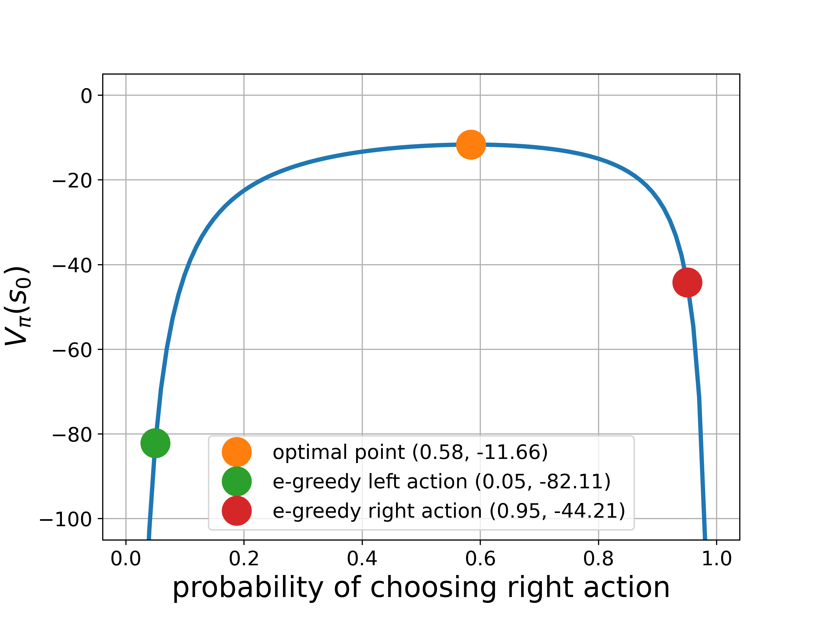
\[V(s_0)=\frac{2(p-2)}{p(1-p)}\]

#return state value of state 0
def v0(p):
    return (2*p-4)/(p*(1-p))

p=np.linspace(0.01, 0.99, 100)
v=v0(p)

op_p=np.argmax(v)
p_op=p[op_p]
v_op=v[op_p]

plt.rcParams['font.size']='14'
plt.figure(figsize=(8,6))
plt.plot(p,v,linewidth=3)
plt.plot(p_op,v_op,'o',markersize=20,label="optimal point ({0:.2f}, {1:.2f})".format(p_op, v_op))
plt.ylim([-105.0,5])

epsilon=0.05

plt.plot(epsilon, v0(epsilon), 'o',markersize=20,
         label="e-greedy left action ({0:.2f}, {1:.2f})".format(epsilon, v0(epsilon)))
plt.plot(1-epsilon, v0(1-epsilon), 'o',markersize=20,
         label="e-greedy right action ({0:.2f}, {1:.2f})".format(1-epsilon, v0(1-epsilon)))
plt.legend()
plt.grid()
plt.ylabel('$V_{\pi}(s_0)$',fontsize=20)
plt.xlabel('probability of choosing right action',fontsize=20)
plt.savefig('egreedy_shortcorridor.png',dpi=350)

The above corresponds to Example 13.1

This experiment shows action-value-based methods have difficulties to find optimal stochastic policy, while policy-based methods can do much better

Implementation of REINFORCE

def policy(theta,phi):
    h=np.dot(theta,phi)
    upper=np.exp(h-np.max(h)) #avoid overflow
    pi=upper/np.sum(upper)

    #keep stochasitc policy with a_min>=0.05
    a_min=np.argmin(pi)
    epsilon=0.05
    if pi[a_min]<epsilon:
        pi[:]=1-epsilon
        pi[a_min]=epsilon

    if np.random.uniform()<=pi[0]:
        return 0,pi
    else:
        return 1,pi

#calculate derivative of log policy
def dlog(phi,a,pi):

    return phi[:,a]-np.dot(phi,pi)

#calculate discounted return in a reversive way
def get_return(rewards,gm):

    R=np.zeros(len(rewards))
    R[-1]=rewards[-1]
    for i in range(2,len(R)+1):
        R[-i]=gm*R[-i+1]+rewards[-i]

    return R

def run_reinforce(lr=2e-4, gm=1, n_eps=1000):

    #initialization of policy parameter theta and state-action feature
    theta=np.array([-1.47,1.47])
    phi=np.array([[0,1],[1,0]])
    #result logging
    s_all,r_all,pi_all=[],[],[]

    for ep in range(n_eps):
        s,stp,done=0,0,False
        #cache for gradient update
        actions,rewards,policies=[],[],[]

        while not done:
            a,pi=policy(theta,phi)
            #pi_all.append(pi)
            s_,r,done=step(s,a)

            actions.append(a)
            rewards.append(r)
            policies.append(pi)

            s=s_
            stp+=1

        R=get_return(rewards,gm)
        #update policy parameter theta
        gmt=1
        for i in range(len(rewards)):
            grad=dlog(phi,actions[i],policies[i])
            theta+=lr*gmt*R[i]*grad
            gmt*=gm

        r_all.append(sum(rewards))
        s_all.append(stp)

    return r_all,s_all#,pi_all

from collections import defaultdict
n_runs=100
lr_all=[2e-4,2e-5,2e-3]
r_res=defaultdict(list) #appendable list

for lr in lr_all:
    for n in range(n_runs):
        r,s,pi=run_reinforce(lr=lr)
        r_res[str(lr)].append(r)   

plt.figure(figsize=(8,6))
for k,v in r_res.items():
    plt.plot(np.array(v).mean(axis=0),label='alpha'+k,linewidth=3)

plt.grid()
plt.axhline(y=-11.6, color='r', linestyle='--',linewidth=3,label='v*(s0)')
plt.legend()
plt.xlabel('Episode')
plt.ylabel('G0 total reward on episode')
plt.savefig('reinforce_shortcorridor.png',dpi=350)

plt.figure(figsize=(8,6))
plt.plot(pi,linewidth=3)
plt.grid()
plt.xlabel('Step')
plt.ylabel('$\pi(s,a)$')
plt.savefig('reinforce_pi_shortcorridor.png',dpi=350)

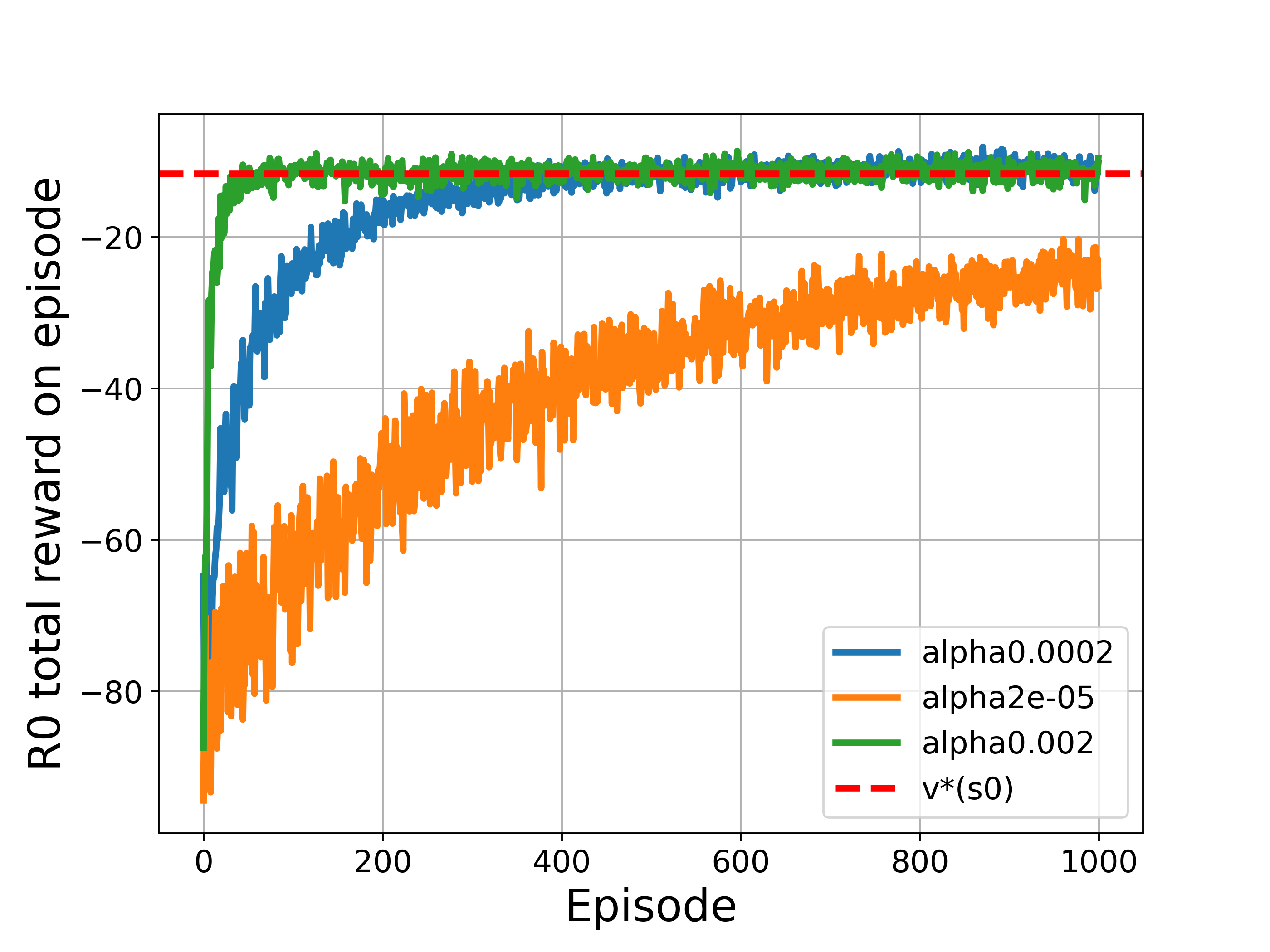
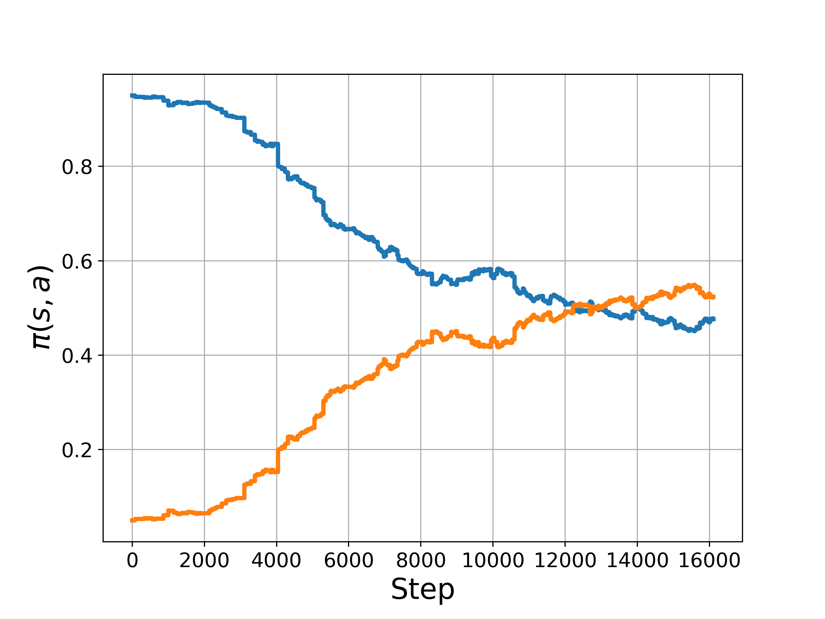
The above corresponds to Figure 13.1

The results show that REINFORCE was able to learn an optimal stochastic policy smoothly, approaching to the optimal value of the starting state

Implementation of REINFORCE with a learned baseline

def run_reinforce_baseline(lr_v=2e-2,lr=2e-3, gm=1, n_eps=1000):

    theta=np.array([-1.47,1.47])
    phi=np.array([[0,1],[1,0]])
    v=0

    s_all,r_all,pi_all=[],[],[]

    for ep in range(n_eps):
        s,stp,r_sum,done=0,0,0,False
        actions,rewards,policies=[],[],[]

        while not done:
            a,pi=policy(theta,phi)
            pi_all.append(pi)
            s_,r,done=step(s,a)

            actions.append(a)
            rewards.append(r)
            policies.append(pi)

            s=s_
            stp+=1

        R=get_return(rewards,gm)

        #update policy parameters
        gmt=1
        for i in range(len(rewards)):
            v+=lr_v*gmt*(R[i]-v)
            theta+=lr*gmt*(R[i]-v)*dlog(phi,actions[i],policies[i])
            gmt*=gm

        r_all.append(sum(rewards))
        s_all.append(stp)

    return r_all,s_all,pi_all

r_res=defaultdict(list)
n_runs=100
for n in range(n_runs):
    r_rf,s_rf,pi_rf=run_reinforce(lr=2e-4)
    r_rfb,s_rfb,pi_rfb=run_reinforce_baseline(lr_v=2e-2,lr=2e-3)
    r_res['reinforce'].append(r_rf)  
    r_res['reinforce-baseline'].append(r_rfb)

plt.figure(figsize=(8,6))
for k,v in r_res.items():
    plt.plot(np.array(v).mean(axis=0),label=k,linewidth=3)

plt.grid()
plt.axhline(y=-11.6, color='r', linestyle='--',linewidth=3,label='v*(s0)')
plt.legend()
plt.xlabel('Episode',fontsize=20)
plt.ylabel('R0 total reward on episode',fontsize=20)
plt.savefig('baseline_shortcorridor.png',dpi=350)

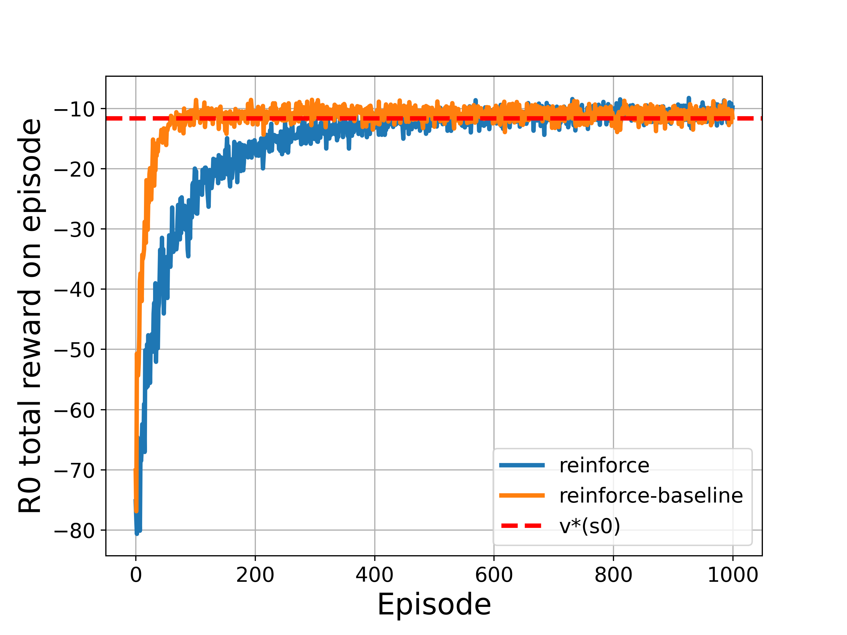
The above corresponds to Figure 13.2

References

Reinforcement Learning an Introduction 2nd edition, Chapter 13 by Sutton and Barto

[1] Peters, Jan, and Stefan Schaal. “Reinforcement learning of motor skills with policy gradients.” Neural networks 21.4 (2008): 682-697.

[2] Schulman, John, et al. “High-dimensional continuous control using generalized advantage estimation.” arXiv preprint arXiv:1506.02438 (2015).

Policy Gradients Methods - Lilian Weng

An Intuitive Explanation of Policy Gradient - Adrien Ecoffet

Going Deeper Into Reinforcement Learning: Fundamentals of Policy Gradients - Daniel Seita

Baseline for Policy Gradients that All Deep Learning Enthusists Must Know

What is the difference between policy gradient methods and actor-critic methods?

Policy-based vs. Value-based - Are they truly different?

ShangtongZhang/reinforcement-learning-an-introduction

Slides and Code

judy_tutorial_basicRL