Distributions I
Keywords
Binomial distributions
Multimonial distributions
for
Discrete random variables
Continuous random variables
Density Estimation
Model p(x) of a random variable x, given a finite set {x_1,x_2,…,x_N} of observations
Assumption: Data points are Independent and Identically Distributed (I.I.D)
Density Estimation is fundamentally ill-posed, cuz there are infinitely many probability distributions that could have given rise to the observed finite data set
Model Selection
The issue of choosing an appropriate distribution for the model
Parametric Distributions
Distributions that are governed by a small number of adaptive parameters, i.e. mean and variance from Gaussian
To determine a target distribution parameters,
In a frequentist treatment, we choose specific values for the parameters by optimizing some criterion, such as the likelihood function
In a Bayesian treatment, we introduce prior distributions over the parameters and use Bayes’ theorem to compute the corresponding posterior distribution given the observed data
Conjugate priors
leads to posterior distribution having the same functional form as the prior, therefore leads to a greatly simplified Bayesian analysis
i.e. the conjugate prior for the parameters of the multinomial distribution is called the Dirichlet distribution
the conjugate prior for the mean of a Gaussian is another Gaussian
Exponential Family
Parametric Density Estimation
Non-Parametric Density Estimation
The distribution typically depends on the size of the data set
Such models still contain parameters, but they control the model complexity rather than the form of the distribution
Sufficient Statistic
A statistic is sufficient for a family of probability distributions if the sample from which it is calculated gives no additional information than does the statistic, as to which of those probability distributions is that of the population from which the sample was taken
Binary Variables
a single binary random variable x∈{0,1}, i.e. coin flipping
x=1   <- heads
x=0   <- tails
Imagine a damaged coin that p(heads)!=p(tails), Say
p(x=1|μ) = μ
p(x=0|μ) = 1-μ

μ - parameter μ∈[0,1]
Bernoulli
Bern(x|μ) = μ^x * (1-μ)^(1-x)

is normalized
mean: E[x]=μ
variance: var[x]=μ(1-μ)
import numpy as np
import matplotlib.pyplot as plt

#hand craft
mu=0.3
plt.bar([0,1],[1-mu,mu],width=0.2)
plt.show()

#scipy
from scipy.stats import bernoulli
import seaborn as sns

data=bernoulli.rvs(size=1000,p=0.3)
ax=sns.distplot(data,kde=False,hist_kws={'linewidth':15})
ax.set(xlabel='Bernoulli',ylabel='Frequency')
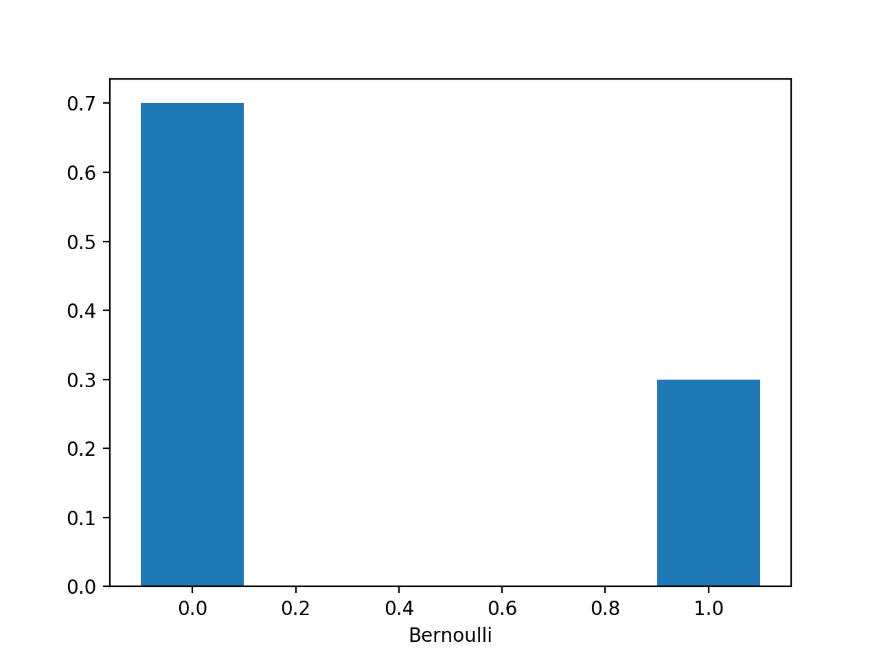
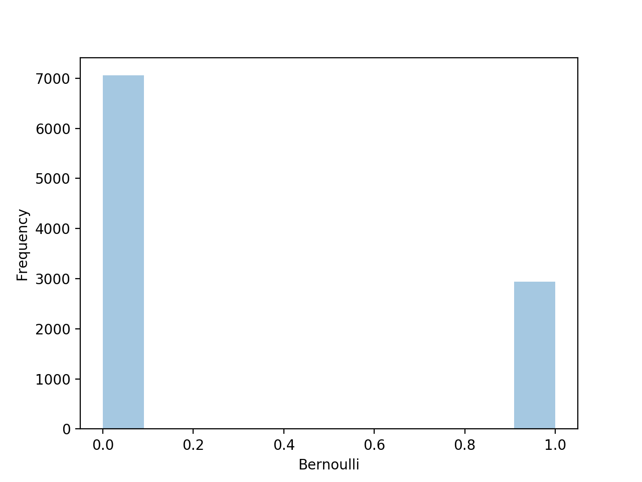
Suppose we have data set D={x_1,…x_N} of observed values of x,
p(D|μ) <- likelihood, a function of μ on the assumption that the observations are drawn independently from p(x|μ)

         N            N
p(D|μ) = ∏ p(x_n|μ) = ∏ μ^x_n * (1-μ)^(1-x_n)
        n=1          n=1
In a frequentist setting, we can estimate a value for μ by maximizing the likelihood or the log-likelihood
ln p(D|μ) = Σ_N ln p(x_n|μ) = Σ_N [x_n*ln(μ)+(1-x_n)ln(1-μ)]
If we set the derivative of ln p(D|μ) w.r.t μ -> 0, we can have the maximum likelihood estimator
dln p(D|μ) / dμ = 0

μ  = 1/N Σ_N x_n      <- sample mean
 ML
If we observe m ‘heads’ in the data set,
μ  = m/N
 ML
Problem:
Suppose, we flip 3 times a coin and happen to observe 3 heads, then
μ  = m/N = 3/3 = 1
 ML
In this case, the maximum likelihood result would predict all future observations should give heads
This is unreasonable, and in fact it is an extreme example of the over-fitting associated with maximum likelihood
Solution:
Introduction of a prior distribution over μ
We can work out the distribution of the number m of observations of x=1, given the data set N
Binomial
In order to obtain the normalization coefficient we not that out of N coin flips, we have to add up all of the possible ways of obtaining m heads,
             (N)
Bin(m|N,μ) = ( ) μ^m*(1-μ)^(N-m)
             (m)

(N)      N!
( ) = --------     <- ways of choosing m objects out of a total N identical objects
(m)   (N-m)!m!

       N
E[m] ≜ Σ m Bin(m|N,μ) = Nμ
      m=0

         N
var[m] ≜ Σ (m-E[m])^2 * Bin(m|N,μ) = Nμ(1-μ)
        m=0
Say N=10, μ=0.25, (flip 10 times coin with μ=0.25, what is the probability of m heads appear)
import numpy as np
import matplotlib.pyplot as plt

#hand craft
def fact(n):
    return np.math.factorial(n)

def binomial(n,m,mu):
    return (fact(n)/(fact(n-m)*fact(m)))*(mu**m)*(1-mu)**(n-m)

n=10
mu=0.25
dist=[]
for m in range(0,10):
    dist.append(binomial(n,m,mu))

plt.bar(range(0,10),dist)
plt.show()

# scipy
from scipy.stats import binom
import seaborn as sns

data=binom.rvs(n=10,p=0.25,size=10000)
ax=sns.distplot(data,kde=False) #norm_hist=True
ax.set(xlabel='Binoamial',ylabel='Frequency')
plt.show()
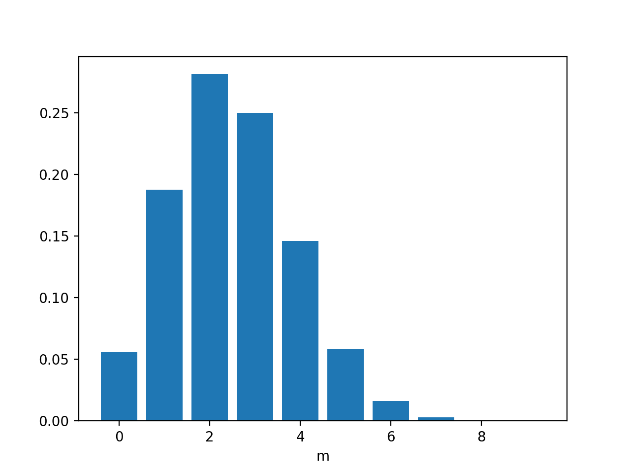
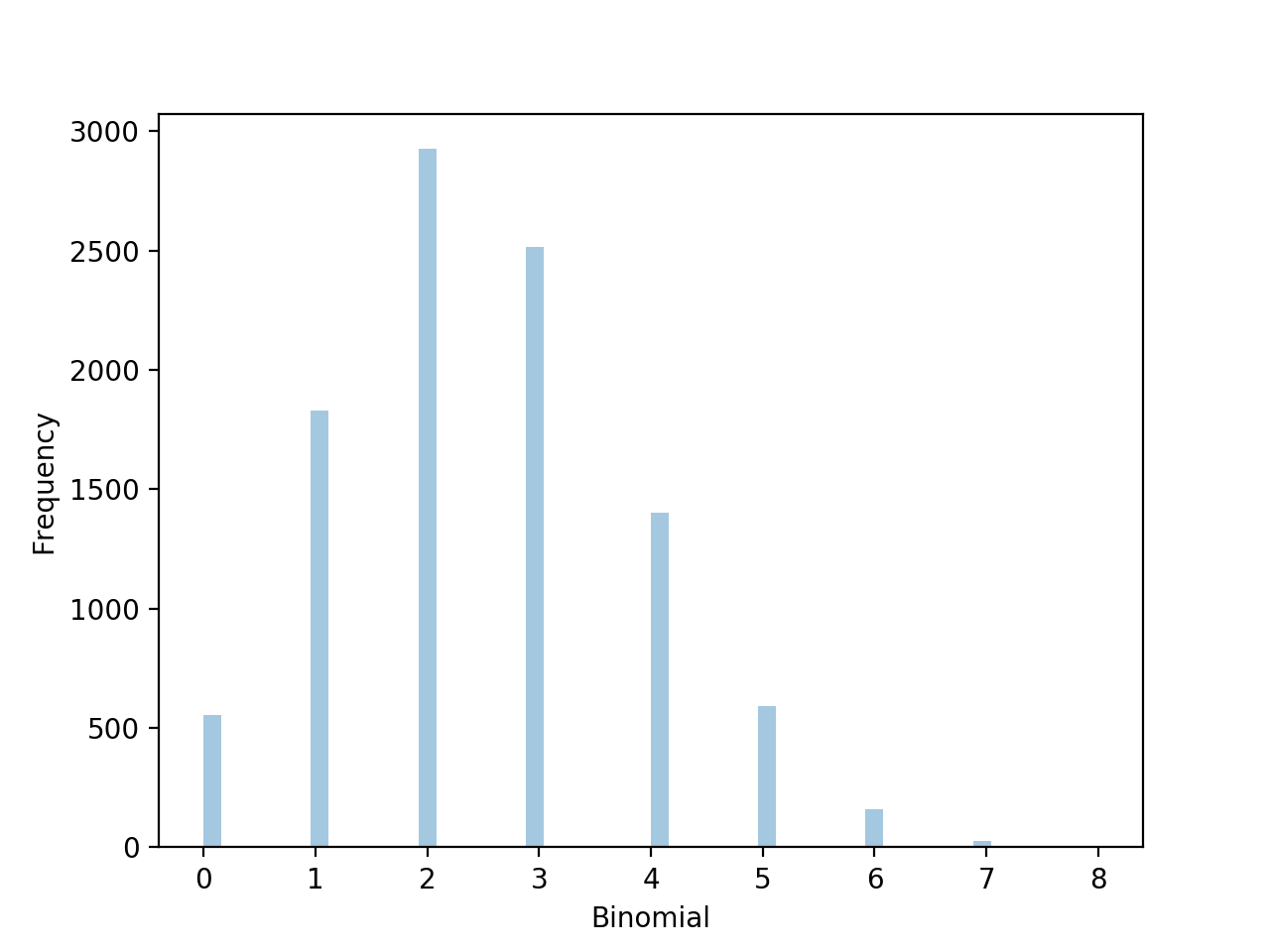
Beta
for being the prior of μ
               Γ(a+b)
Beta(μ|a,b) = -------- μ^(a-1) * (1-μ)^(b-1)
              Γ(a)Γ(b)

Γ(x) - the gamma function

       ∞
Γ(x) ≜ ∫ u^(x-1) * e^(-u) du
       0

Γ(x+1) = xΓ(x)

                 Γ(a+b)
the coefficient --------- ensures the beta distribution is normalized
                 Γ(a)Γ(b)

1
∫ Beta(μ|a,b) dμ = 1
0

         a
E[μ] = -----
        a+b

               ab
var[μ] = --------------
         (a+b)^2(a+b+1)

a,b - hyperparameters, controls the distribution of parameter μ
Generate data
from scipy.stats import beta
import seaborn as sns

data=beta.rvs(0.1,0.1,size=10000)
sns.distplot(data,bins=100)
data=beta.rvs(1,1,size=10000)
sns.distplot(data,kde=False,bins=100)
data=beta.rvs(2,3,size=10000)
sns.distplot(data,kde=False,bins=100)
data=beta.rvs(8,4,size=10000)
sns.distplot(data,kde=False,bins=100)
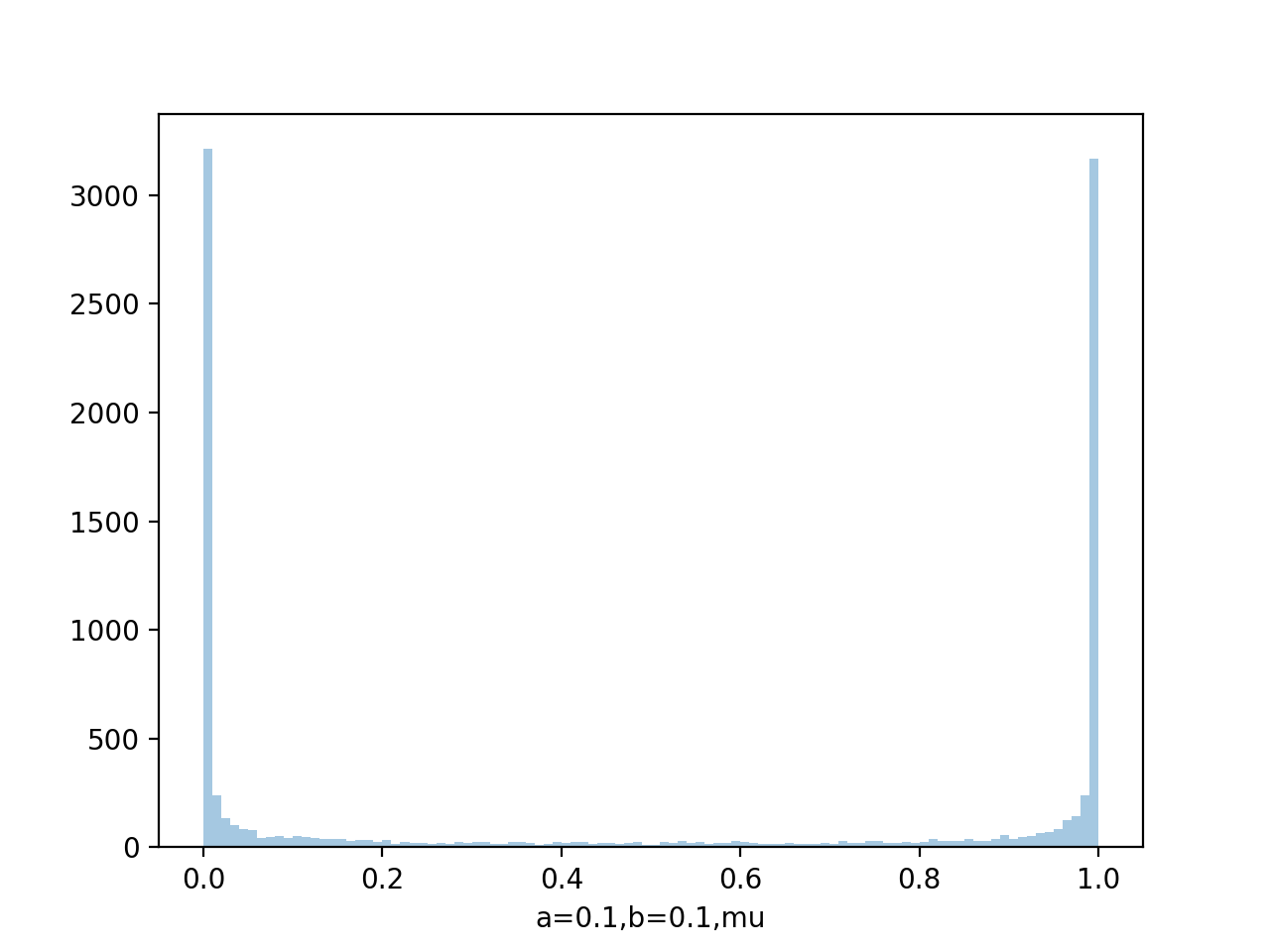
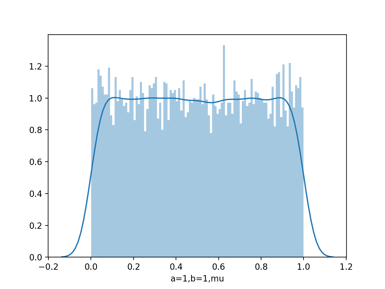
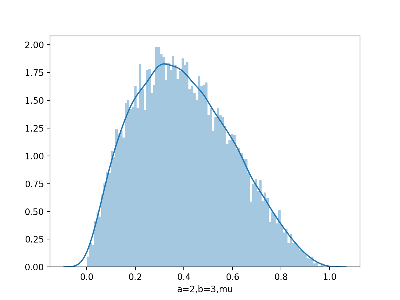
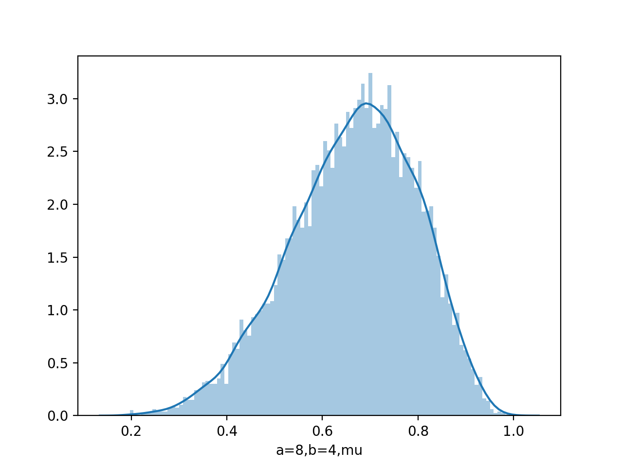
Draw pdf
x=np.linspace(0,1,size=1000)
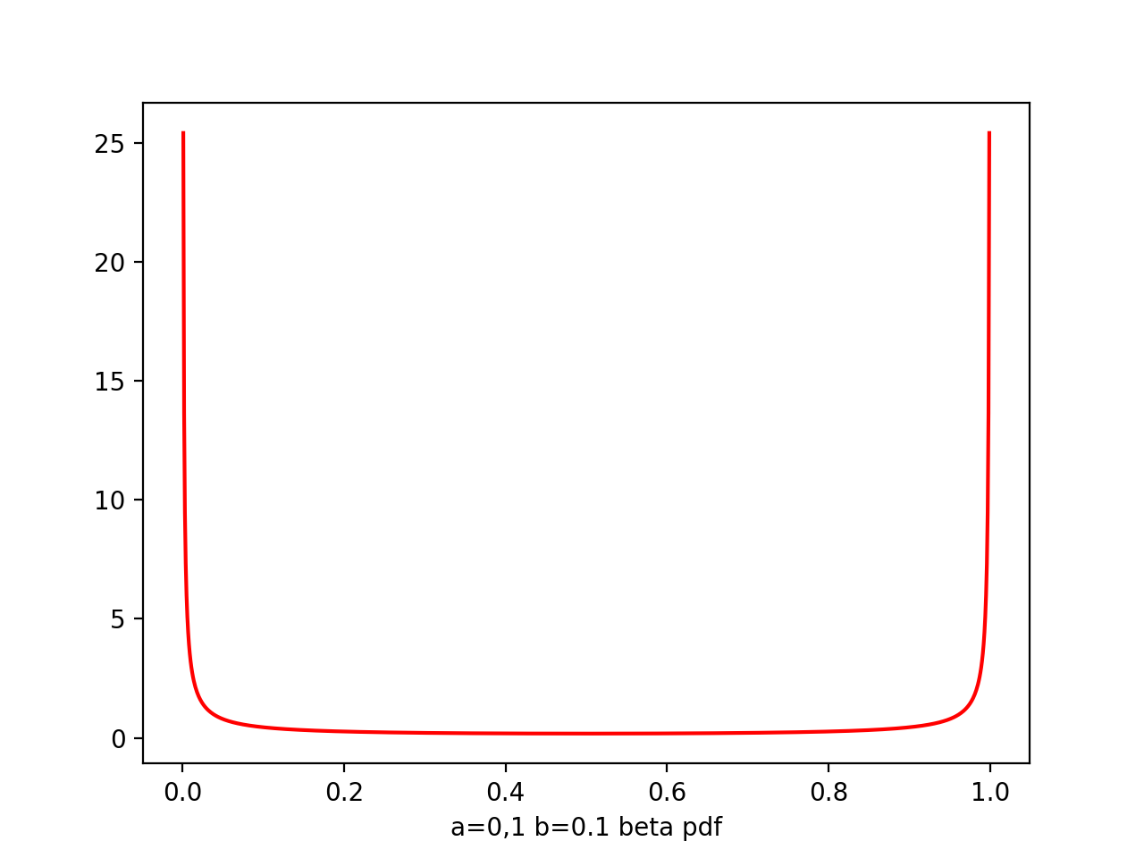
plt.plot(x,beta.pdf(x,0.1,0.1),'r')
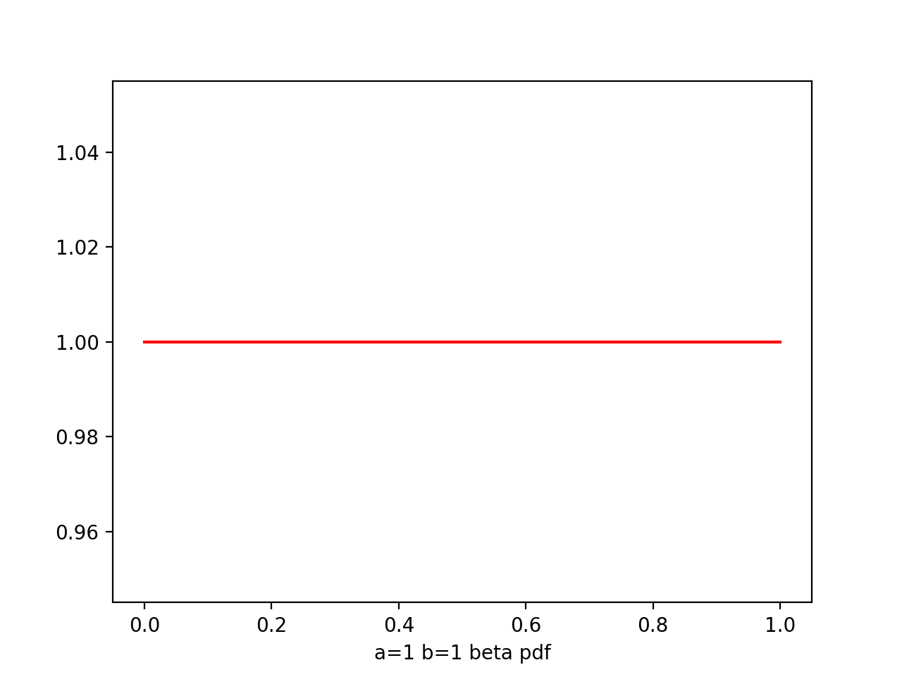
plt.plot(x,beta.pdf(x,1,1),'r')
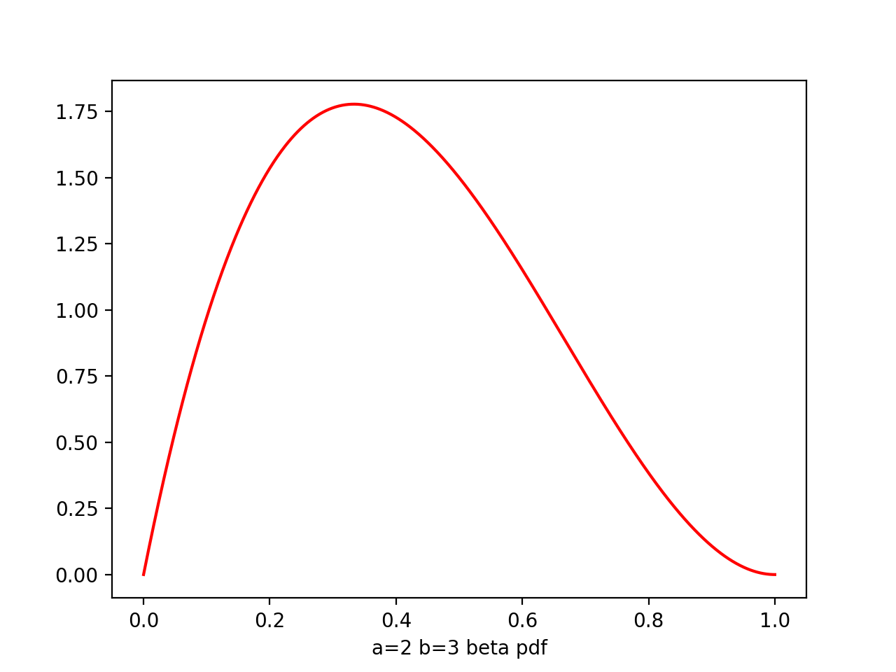
plt.plot(x,beta.pdf(x,2,3),'r')
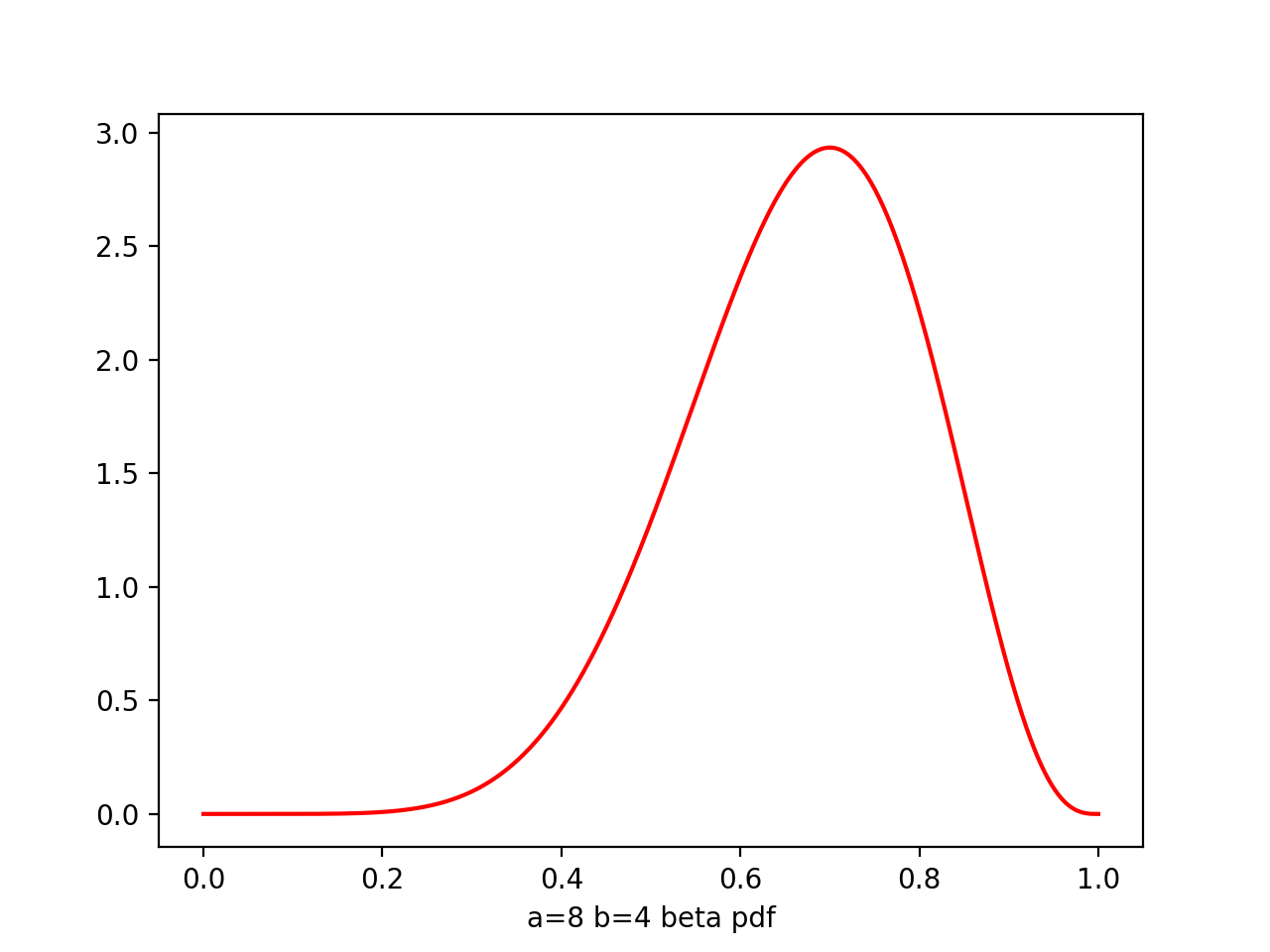
plt.plot(x,beta.pdf(x,8,4),'r')
A Whole Bayesian View
The posterior of μ is obtained by multiplying the beta prior and the binomial likelihood
prior:
               Γ(a+b)
Beta(μ|a,b) = -------- μ^(a-1) * (1-μ)^(b-1)
              Γ(a)Γ(b)

likelihood:

             (N)
Bin(m|N,μ) = ( ) μ^m * (1-μ)^(N-m)
             (m)

posterior: (keeping only the factors dependent on μ)

p(μ|m,N,a,b) ∝ μ^(m+a-1) * (1-μ)^(N-m+b-1)
The posterior has the same functional as the prior, reflecting the conjugacy properties of the prior w.r.t the likelihood function
Then, the normalization coefficient is
                  Γ(N+a+b)
p(μ|m,N,a,b) = -------------- μ^(m+a-1) * (1-μ)^(N-m+b-1)
               Γ(m+a)Γ(N-m+b)
We can simply interpret a,b are effective numbers of observations of x=1 and x=0
i.e. prior ~ Beta(a=2,b=2), likelihood ~ Bin(N=m=1) => post ~ Beta(a=3,b=2)
x=np.linspace(0,1,num=1000)
a=2
b=2
plt.plot(x,beta.pdf(x,a,b),'r')
N=1
m=1
plt.plot(x,x,'b')
a=3
b=2
plt.plot(x,beta.pdf(x,a,b),'r')
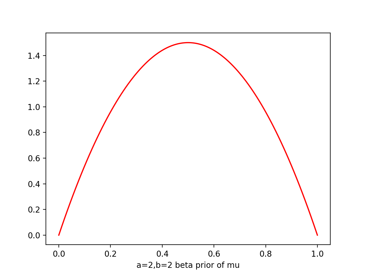
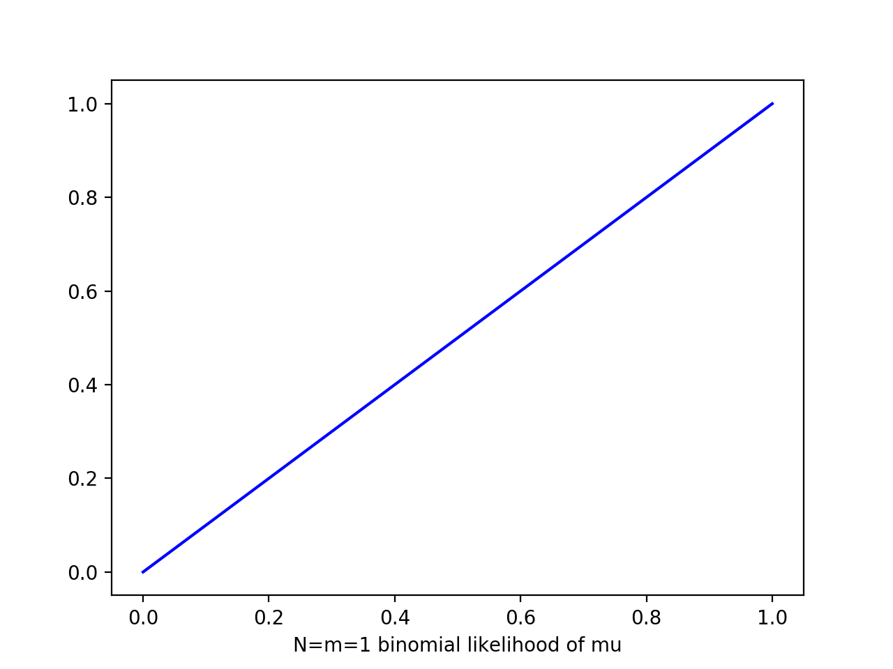
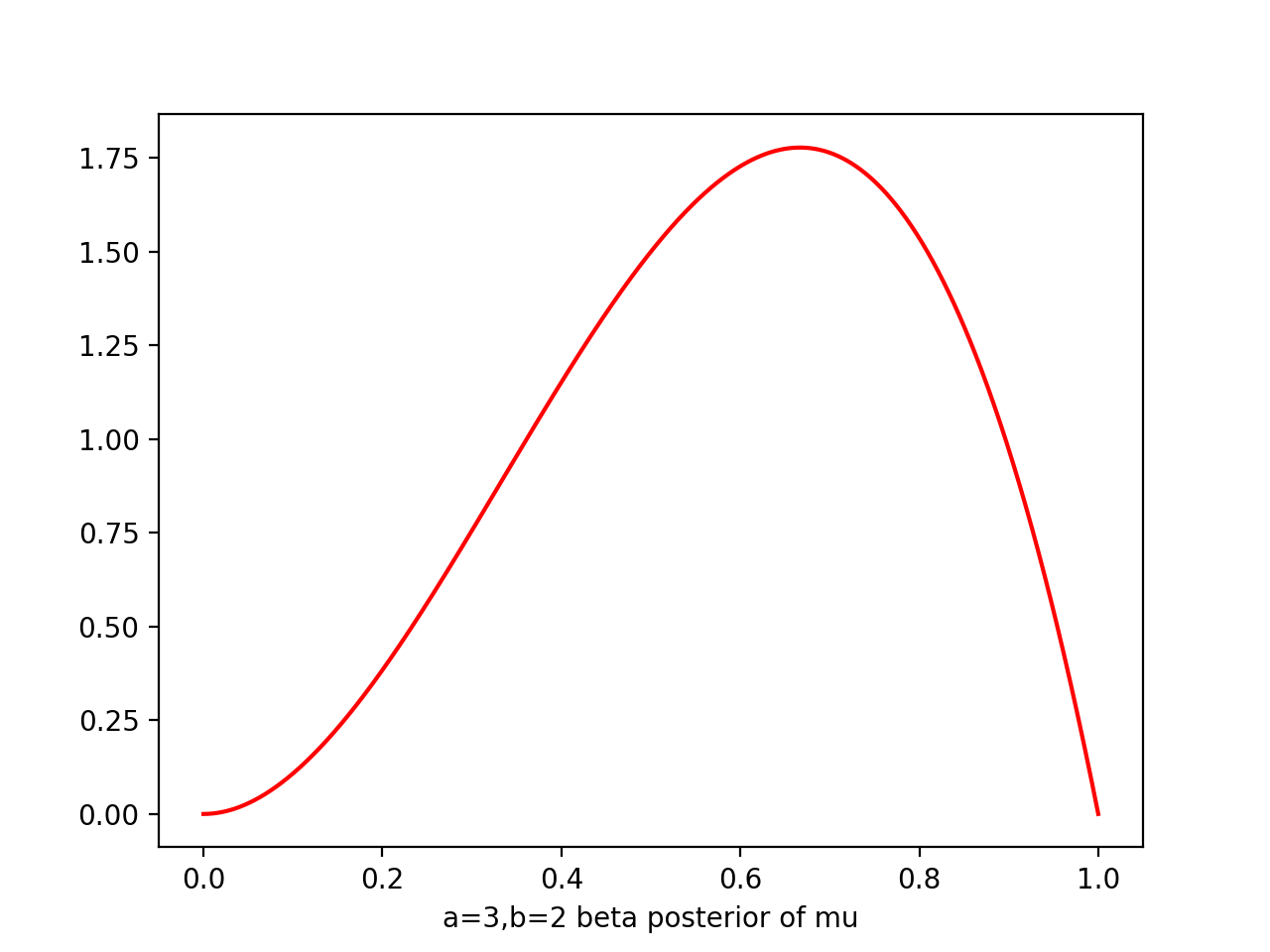
At each stage, the posterior is beta given current observed values of 1s and 0s generated by a,b
observe one more x=1 simply corresponds to incrementing a by 1, and x=0 of b by 1
Sequential Approach
Sequential approaches make use of observations one at a time, or in small batches, then discard them before the next observations are used
(+) real time streaming
(+) do not require the whole data set
(+) can be useful for large data sets
If we evaluate the predictive distribution of x given the observed data set D
           1                    1
p(x=1|D) = ∫ p(x=1|μ)p(μ|D)dμ = ∫ μp(μ|D)dμ = E[μ|D]
           0                    0

             a                         Γ(N+a+b)
use E[μ] = ----- and p(μ|m,N,a,b) = -------------- μ^(m+a-1) * (1-μ)^(N-m+b-1) for p(μ|D)
            a+b                     Γ(m+a)Γ(N-m+b)

              m+a     -> correspond to x=1
p(x=1|D) = ---------
             N+a+b

if N->∞,   p(x=1|D) =  m/N           = μ_ML
(infinite            (a,b are          (exactly the maximum likelihood result)
 large                small enough
 data set)            to be ignored)

if N is finite, p(x=1|D) lies between the prior mean E[μ]=a/(a+b) and maximum likelihood estimate 1/N Σ_N x_n
From figure of beta a,b from (0.1,0.1) to (8,4), we see as the number of observations increases, so the posterior distribution becomes more sharply peaked
This can also be seen from var[μ]=ab/(a+b)^2(a+b+1), in which we see the variance goes to zero for a->∞ or b->∞
AKA a general property of Bayesian learning, that as we observe more and more data, the uncertainty represented by the posterior distribution will steadily decrease
Proof of this property
Reference
Bishop Chapter 2 Probability Distributions
Probability Distributions in Python with SciPy and Seaborn
Binomial Distribution: Formula, What it is and How to use it
