Markov Chain Monte Carlo
Motivation
It turns out sampling from any but the most basic probability distribution is a difficult task. Methods include
- inverse transform sampling (IRT)
- rejection sampling (RS)
IRT requires the cumulative distribution function aka normalization constant, which can be obtained by numerical integration.
(-) however, it quickly gets infeasible with an increasing number of dimensions
RS doesnt require a normalized distribution
(-) however, efficiently implementing it requires a good deal of knowledge about the distribution of interest
(-) it suffers strongly from the curse of dimension
Markov Chain Monte Carlo refers to a class of methods doing so as well, namely for sampling from a probability distribution in order to construct the most likely distribution.
For example, we cannot directly calculate the logistic distribution, so instead we generate thousands of values — called samples — for the parameters of the function to create an approximation of the distribution.
The more samples generated, the closer and closer the approximation gets to the actual true distribution.
Monte Carlo
Monte Carlo refers to a general technique of using repeated random samples to obtain a numerical answer.
It can be thought of as carrying out many experiments, each time changing the variables in a model and observing the response.
By choosing random values, we can explore a large portion of the parameter space, the range of possible values for the variables.
Markov Chain
A Markov Chain is a process where the next state depends only on the current state.
(+) it’s memoryless because only the current state matters and not how it arrived in that state.
Markov Chain Monte Carlo
MCMC is a method that repeatedly draws random values for the parameters of a distribution based on the current values. Each sample of values is random, but the choices for the values are limited by the current state and the assumed prior distribution of the parameters.
MCMC can be considered as a random walk that gradually converges to the true distribution.
Markov Chain Example
In order to sample from a distribution p(x), a MCMC algorithm construts and simulates a Markov Chain whose stationary distribution is p(x), meaning that, after an initial ‘burn-in’ phase, the states of that Markov Chain are distributed according to p(x). We thus just have to store the states to obtain samples from p(x).
Let’s consider a discrete state space and discrete time,
Markov Chain maintains a transition operator T(x’|x) which gives you the probability of being in state x’ at time t+1 that the chain is in state x at time t.
Let’s assume three weather states {‘sunny’,’cloudy’,’rainy’}
The transition matrix is:
T=[[0.6,0,3,0.1],
   [0.3,0.4,0.3],
   [0.2,0.3,0.5]]
which means
if current,next -> sunny cloudy rainy
   sunny           [0.6,  0,3,   0.1]
   cloudy          [0.3,  0.4,   0.3]
   rainy           [0.2,  0.3,   0.5]
empricial probability:
states=[0,0,0,0,1,1,2,1,0,2,1...]
interval=range(1,20000,5)=[1,6,11,16,...], len=4000
x=1,6,11,16,...
take x=11
count0=5, p0=5/11
count1=4, p1=3/11
count2=2, p2=2/11
from __future__ import division
import numpy as np

T=np.array([[0.6,0.3,0.1],[0.3,0.4,0.3],[0.2,0.3,0.5]])
n_steps=20000
n_states=3
states=[0]

for i in range(n_steps):
    states.append(np.random.choice((0,1,2),p=T[states[-1]]))

states=np.array(states)
emp_prob=[]

interval=range(1,n_steps,5) #sample interval
for i in range(n_states):
    emp_prob.append([np.sum(states[:x]==i)/x for x in interval])#empirical probability
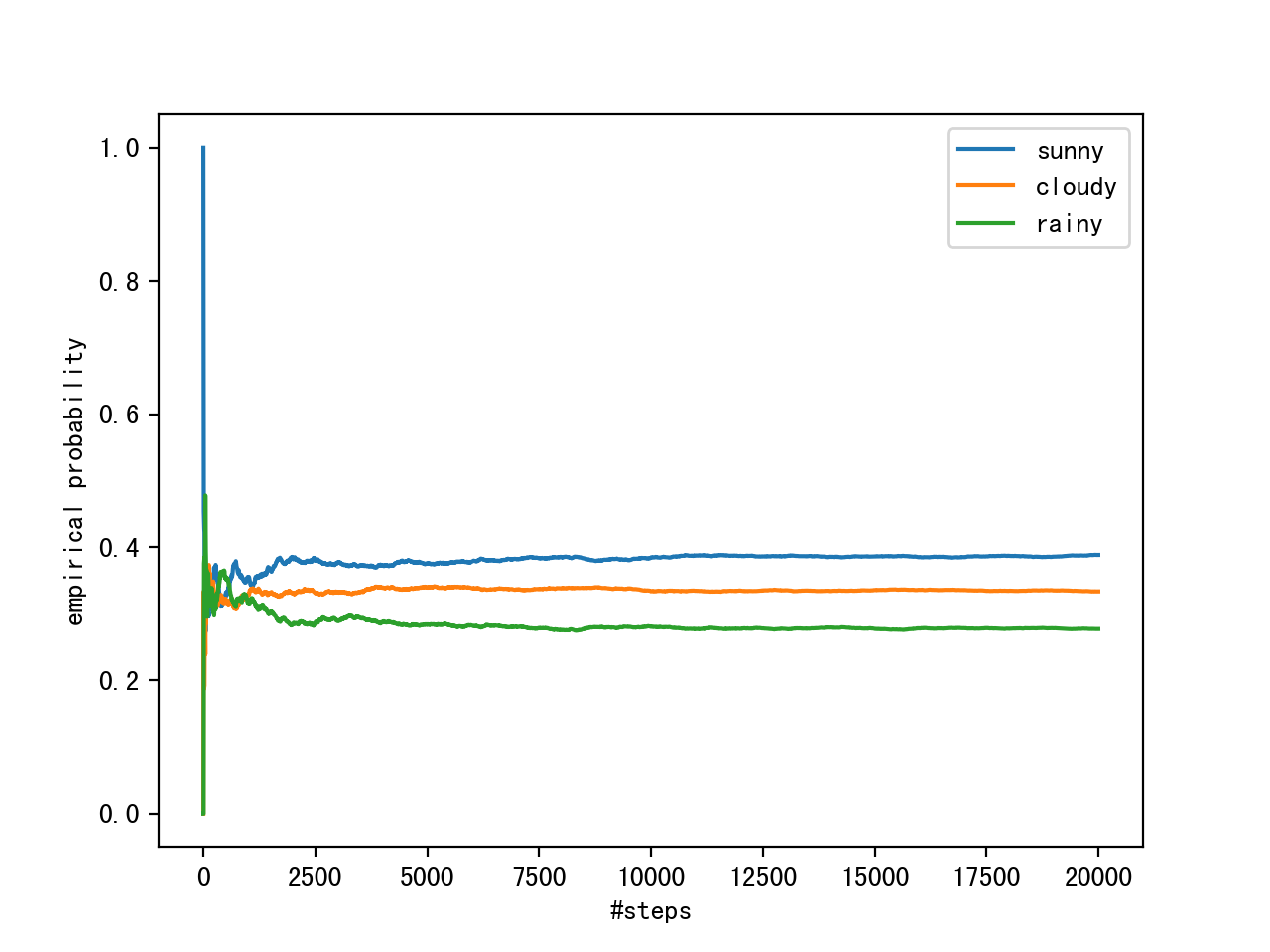
We can observe the convergence of the Markov chain to its stationary distribution by calculating the empirical probability for each of the states as a function of chain length.
Metropolis-Hastings
In discrete case, we call T a transition matrix.
In continuous case, we call T a transition kernel.
The Goal is to design the transition kernel T
Split T(x’|x) into two parts:
- a proposal step
- an acceptance/rejection step
Recall the original distribution is defined by p(x)
The proposal step features a proposal distribution q(x’|x), where we can sample possible next states of the chain
We can choose q arbitrarily, however, we need to design the q such that samples from it are both as little correlated with the current state as possible and have a good chance of being accepted in the acceptance step
The acceptance step corrects for the error introduced by proposal states drawn from q!=p
It involves calculating an acceptance probability p_acc(x’|x) and accepting the proposal x’ with that probability as the next state in the chain
Steps:
- a proposal point x’~q(x’|x)
- x’ is accepted with p_acc(x’|x), or is rejected with 1-p_acc(x’|x)
Therefore, we have T(x’|x)=q(x’|x)*p_acc(x’|x)
A sufficient condition for Markov Chain to have p as its stationary distribution is:
the transition kernel obeying detailed balance: p(x)T(x’|x)=p(x’)T(x|x’)
meaning: the probability of being in a state x and transitioning to x’ must be equal to the probability of the reverse process, namely, being in state x’ and transitioning to x.
For the two-part transition kernel to obey detailed balance, we need to choose p_acc correctly, one possibility is the Metropolis Acceptance criterion:
                     p(x')q(x|x')
p_acc(x'|x)=min { 1, ------------ }
                     p(x)q(x'|x)
where the unknown constant cancels out. This makes the algorithm work for unnormalized distributions
Often, symmetric proposal distributions with q(x|x’)=q(x’|x), then we have
                      p(x')
p_acc(x'|x)=min { 1, ------ }
                      p(x)
Then
           q(x'|x)p_acc(x'|x)   :  x'!=x
T(x'|x)={
           1-∫dx'q(x'|x)p_acc(x'|x)  :  x'==x
Implementation
step 1: set a log-probability of the p we want to sample from, without normalization constants, say a standard Gaussian
def log_prob(x):
    return -0.5*np.sum(x**2)
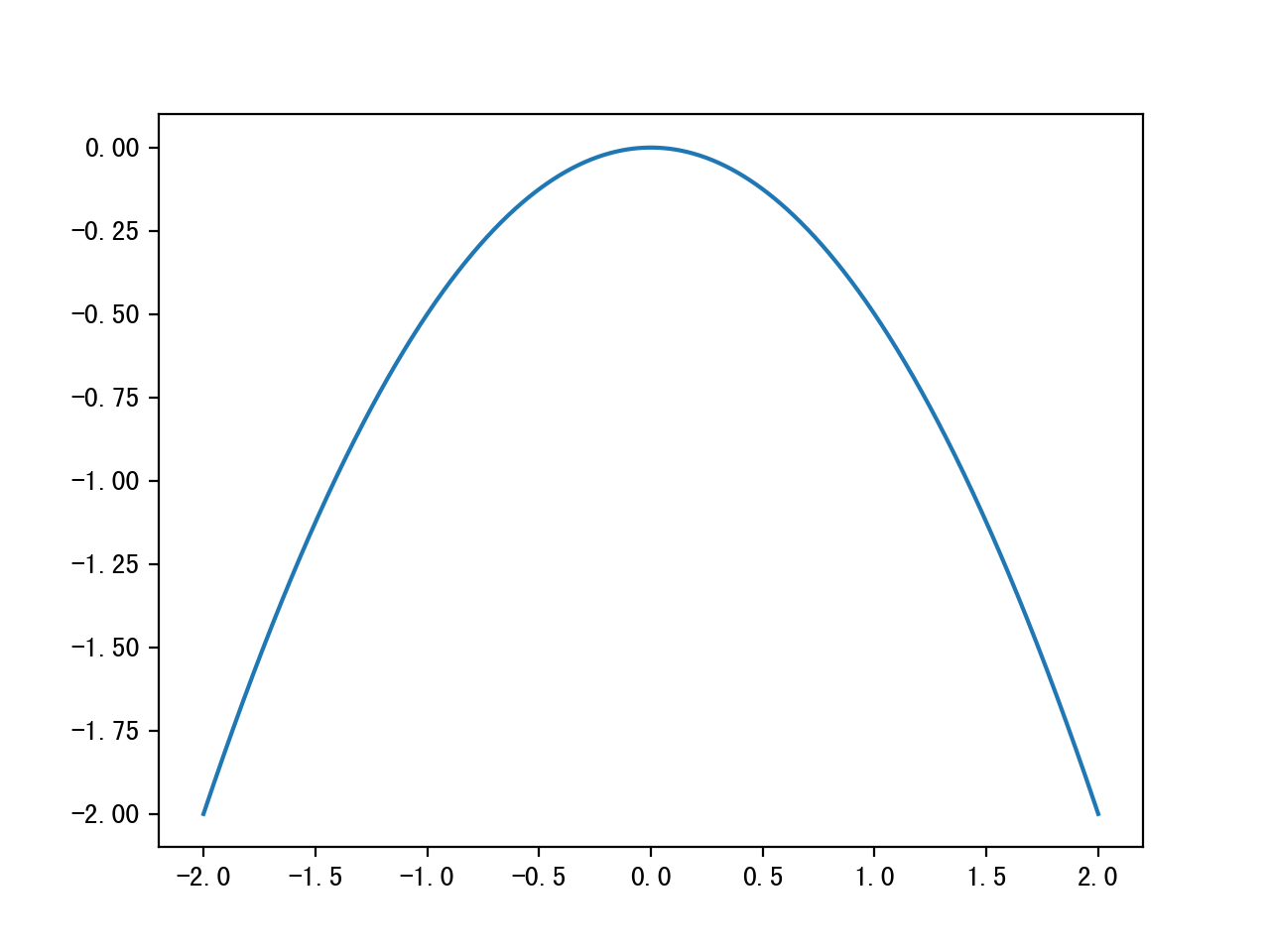
step 2: choose a symmetric proposal distribution, a naive approach is just take the current state x and pick a proposal from U(x-∆/2,x+∆/2), where ∆ is a step size
def proposal(x,delta):
    return np.random.uniform(low=x-0.5*delta,high=x+0.5*delta,size=x.shape)
step 3: calculate our acceptance probability
def p_acc_MH(x_new, x_old, log_prob):
    return min(1,np.exp(log_prob(x_new)-log_prob(x_old)))
brief implementation of a Metropolis-Hastings sampling step:
def sample_MH(x_old, log_prob, delta):
    x_new=proposal(x_old,delta)
    accept=np.random.random()<p_acc_MH(x_new,x_old,log_prob)
    if accept:
        return accept, x_new
    else:
        return accept, x_old
build the Markov Chain:
def build_MH_chain(init,delta,n_total,log_prob):
    n_accepted=0
    chain=[init]
    for i in range(n_total):
        accept,state=sample_MH(chain[-1],log_prob,delta)
        chain.append(state)
        n_accepted+=accept

    acceptance_rate=n_accepted/float(n_total)
    return chain, acceptance_rate
TESTING!!
init=np.array([2.0])
delta=3.0
n=10000

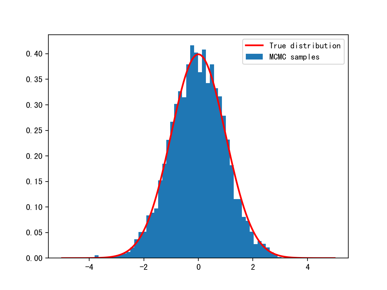
chain, acceptance_rate=build_MH_chain(init,delta,n,log_prob)
chain=[s for s, in chain]

Z,_=quad(lambda x:np.exp(log_prob(x)),-np.inf,np.inf)
#Z=2.50662827463
x=np.linspace(-5,5,1000)
y=[np.exp(log_prob(i))/Z for i in x]

plt.hist(chain[500:],bins=50,density=True, label='MCMC samples')
plt.plot(x,y,'r',linewidth=2, label='True distribution')
plt.legend()
Motivation from Bayesian
Bayes Formula
        p(x|θ)p(θ)
p(θ|x)=------------
           p(x)
p(θ|x) - the probability of our model parameters θ given the data x
p(θ) - prior: what we think about θ before we have seen any data
p(x|θ) - likelihood: how we think our data is distributed
p(x) - the evidence: the evidence that the data x was generated by this model
p(x)=∫ p(x,θ) dθ
     θ
difficulty: p(x) can not be computed in a closed-form way
Bayesian Example
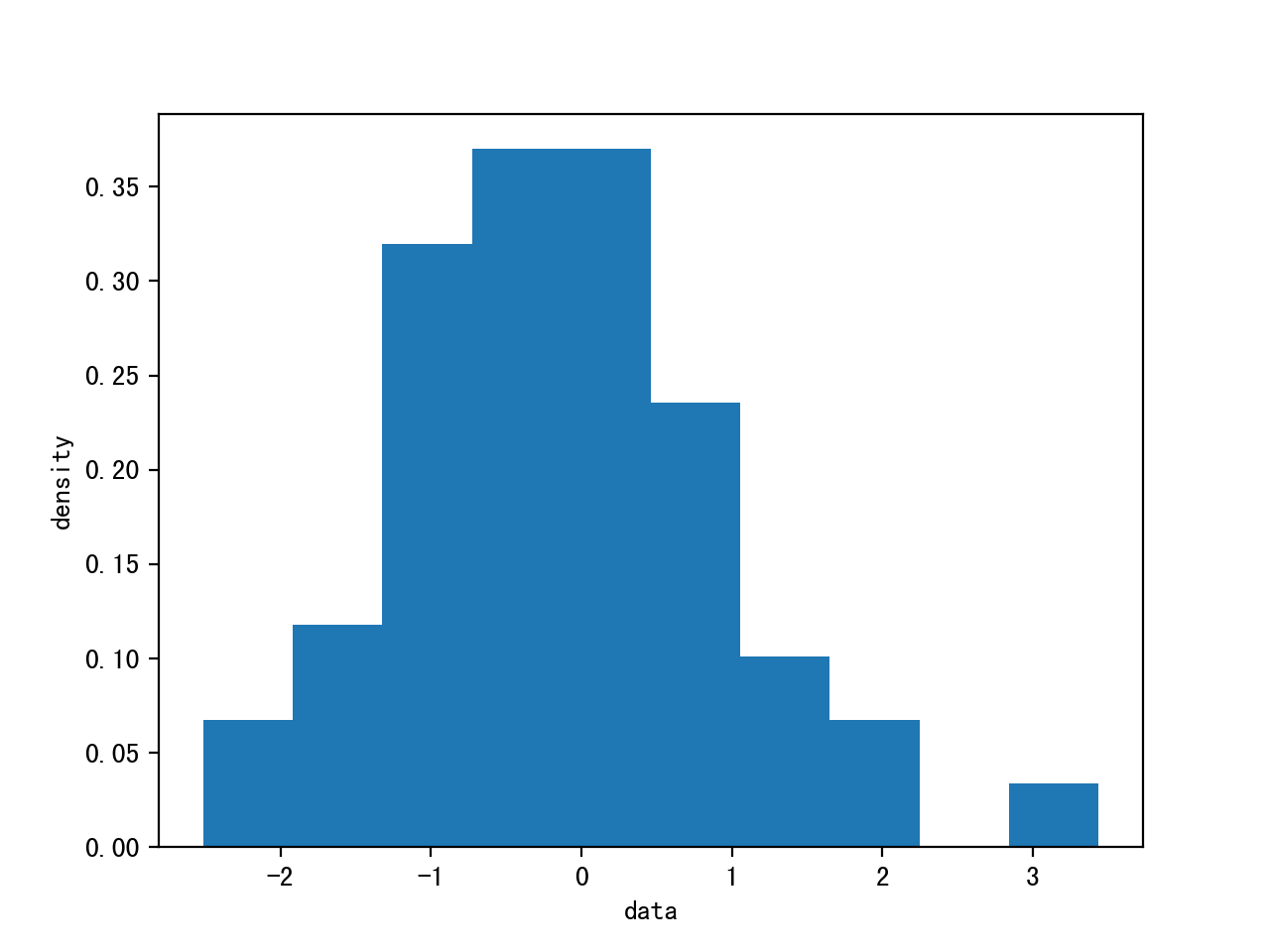
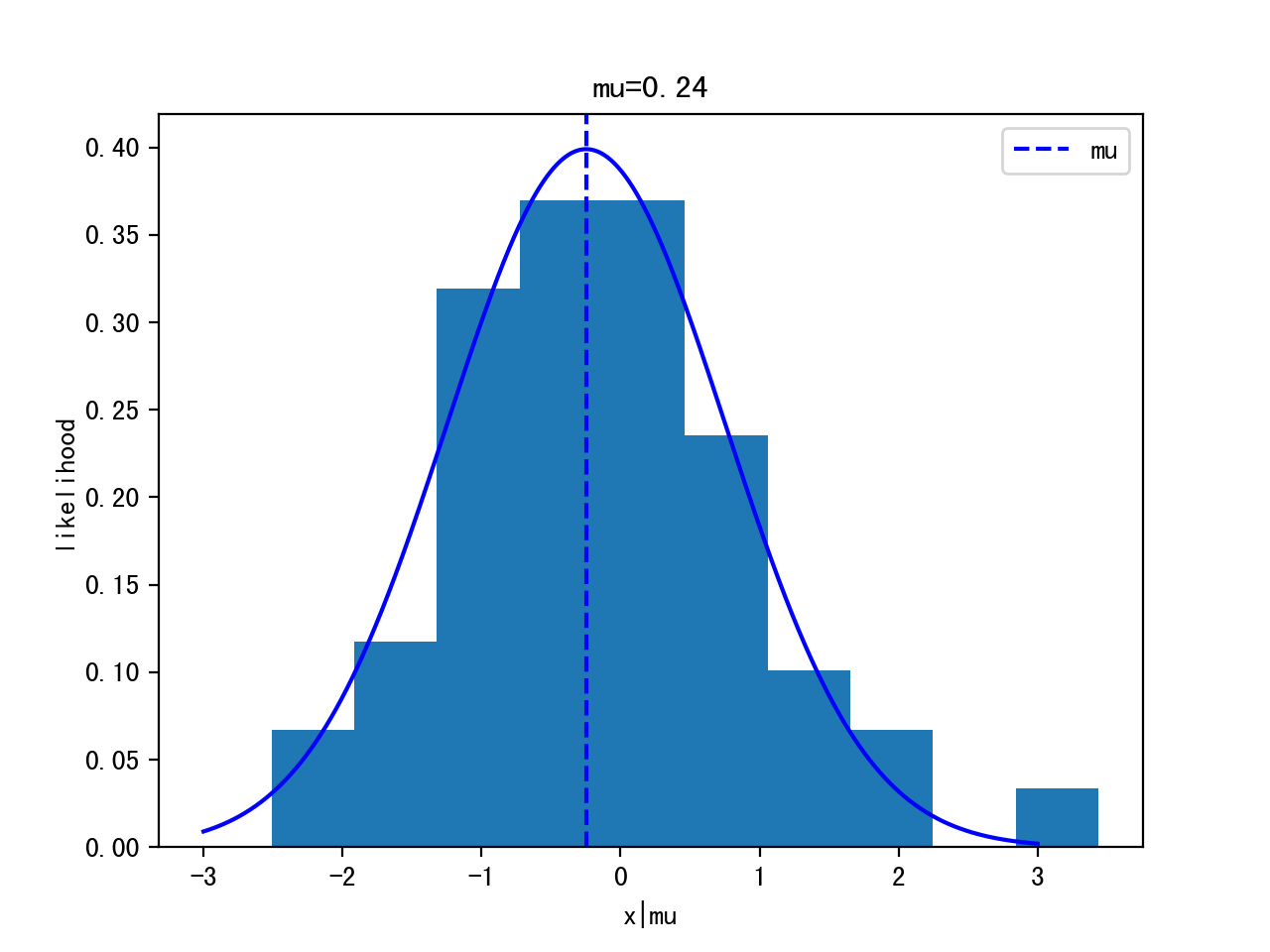
Given 100 data points, estimate the posterior of the mean.
(The data is generated by Gaussian distribution mean=0, variance=1)
import numpy as np
import matplotlib.pyplot as plt

data=np.random.randn(100)
plt.hist(data)
Steps:
- assume data is normal distributed: p(x|θ) ~ Gaussian(μ,σ) - mean and standard deviation, assume σ=1 is known for simplicity
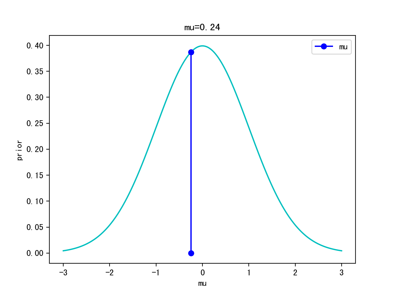
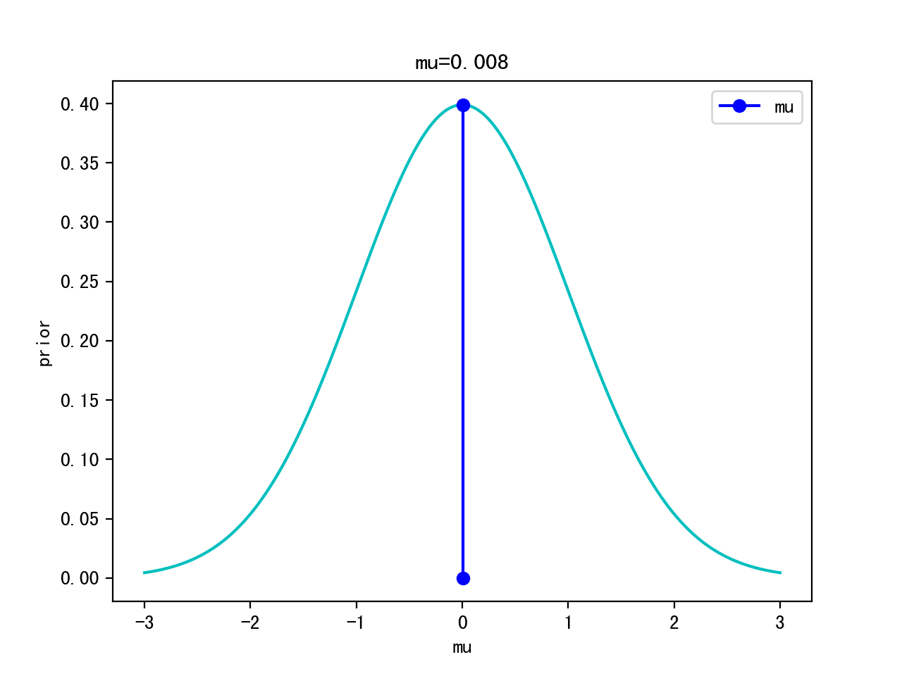
- choose a prior: p(θ) ~ Gaussian(0,1) for simplicity
Model:
p(x|θ): p(x|μ,σ)=p(x|μ,1) -> p(x|μ) ~ Gaussian (μ,1) <- likelihood
                                      Gaussian (μ,σ)
p(θ):   p(μ,σ)=p(μ,1)     -> p(μ)   ~ Gaussian (0,1) <- prior
                                      Gaussian (ρ,τ) (mean,std)
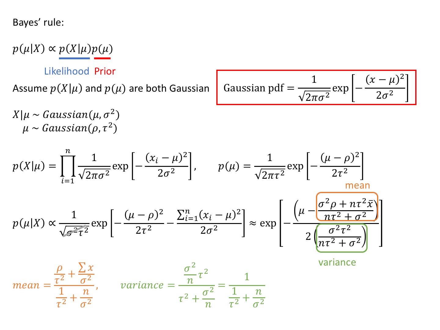
Analytical Solution
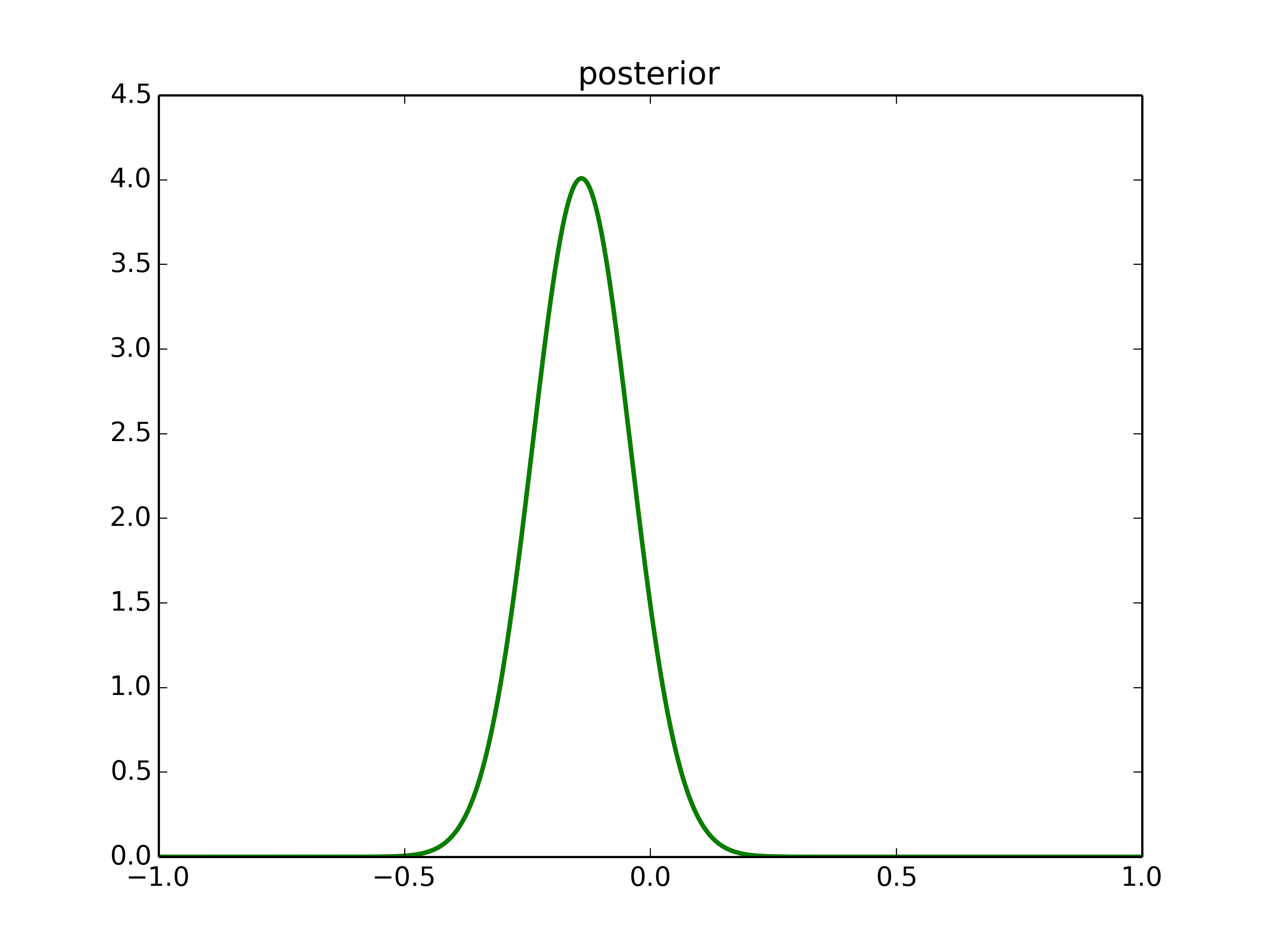
Can compute the posterior analytically, because for a Gaussian likelihood with known standard deviation, the Gaussian prior for μ is conjugate
=> the posterior for μ is Gaussian as well
Conjugate
posterior and prior will be the same distribution
import numpy as np
import matplotlib.pyplot as plt
from scipy.stats import norm

def gaussian(x,mu,sig):
    pdf=(1./(sig*np.sqrt(2*np.pi))*np.exp(-(x-mu)**2/(2*sig**2)))
    return pdf

def posterior_analytical(data,rho,tau): #mu,sig prior parameters
    n=len(data)
    sig=1.
    mu_post=(rho/tau**2+data.sum()/sig**2)/(1./tau**2+n/sig**2)
    sig_post=(1./tau**2+n/sig**2)**-1
    return mu_post,sig_post

data=np.random.randn(100)
x=np.linspace(-1,1,500)

mu_post,sig_post=posterior_analytical(data,0.,1.) #mu_0,sig_0
pdf1=gaussian(x,mu_post,np.sqrt(sig_post)) #by hand
pdf2=norm(mu_post,np.sqrt(sig_post)).pdf(x) #by library, same way to get pdf

plt.plot(x,pdf1,'r',linewidth=2)
plt.plot(x,pdf2,'g',linewidth=2)
However, the prior wasn’t conjugate and we couldn’ sovle this by hand is usually the case.
MCMC sampling
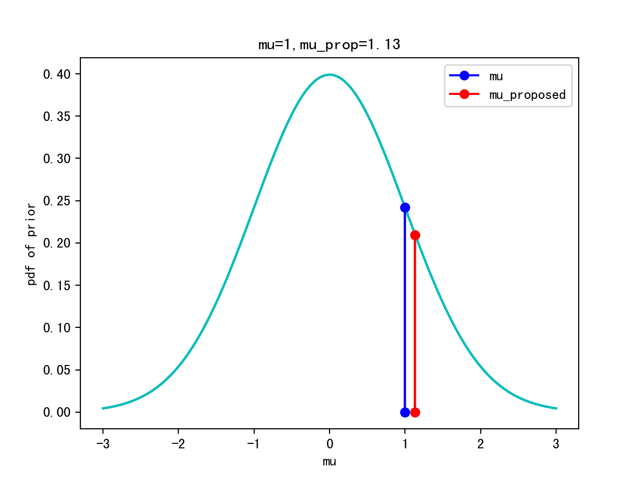
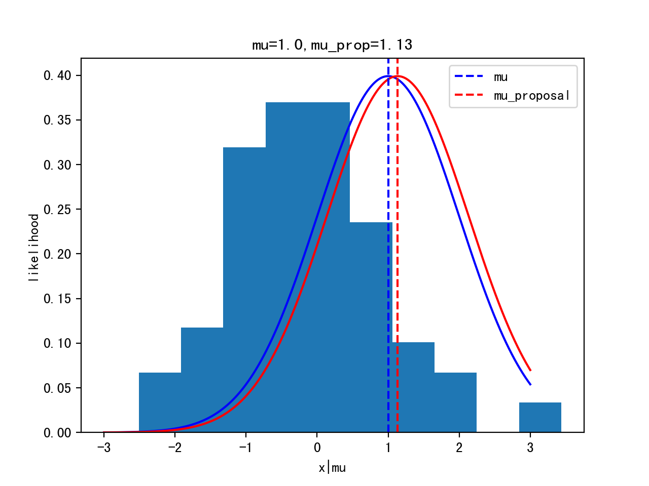
Start sampling: μ = 1.
Proposal: μ’ ~ Gaussian(μ,width)
Acceptance:
        p(μ'|x)   p(x|μ')p(μ')     prod(G(μ',1).x)G(ρ,τ).μ'
p_acc = ------- = ------------- = -------------------------
        p(μ|x)     p(x|μ)p(μ)       prod(G(μ,1).x)G(ρ,τ).μ
This way, we are visiting regions of high posterior probability relatively more often than those of low posterior probability.
def sampler(data,n_samples=100,mu=.5,witdh=.5,mu_pri=0,std_pri=1.):
    mu=mu
    posts=[mu]
    n_accepted=0

    for i in range(n_samples):
        mu_prop=norm(mu,width).rvs()

        lh=norm(mu,1).pdf(data).prod()  # likelihood should be all producted up
        lh_prop=norm(mu_prop,1).pdf(data).prod()

        pri=norm(mu_pri,std_pri).pdf(mu)
        pri_prop=norm(mu_pri,std_pri).pdf(mu_prop)

        post=lh*pri
        post_prop=lh_prop*pri_prop

        p_acc=post_prop/post

        accept=np.random.rand()<p_acc

        if accept:
            mu=mu_prop
            n_accepted+=1
            posts.append(mu)

    return n_accepted/n_samples, np.array(posts)
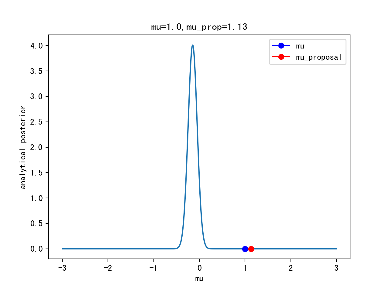
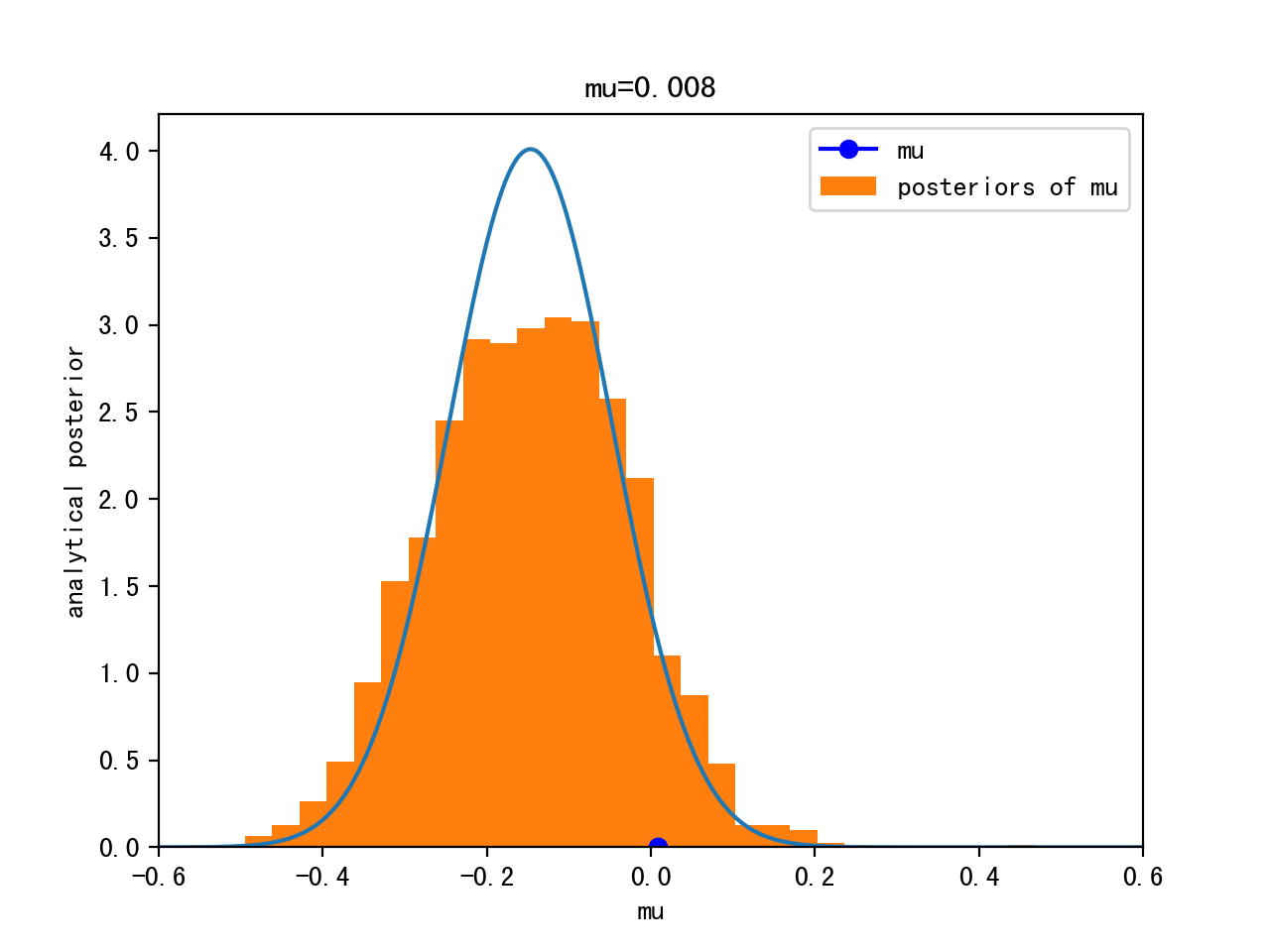
Iteration 0:
Itertation 10:
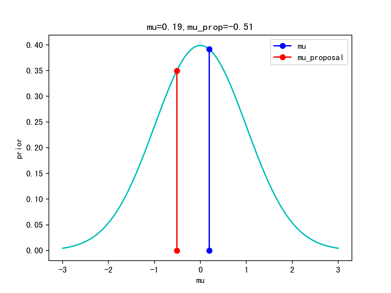
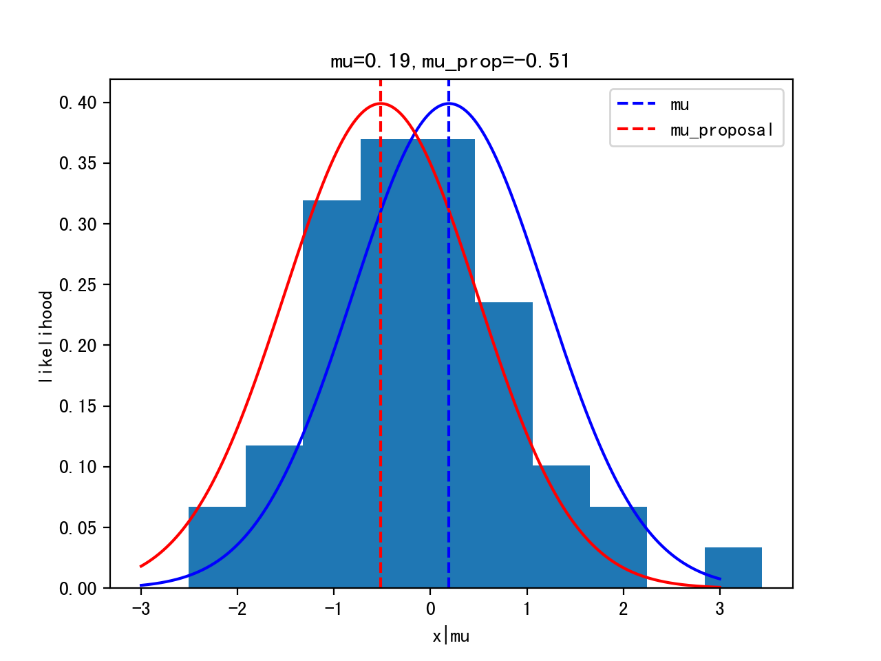
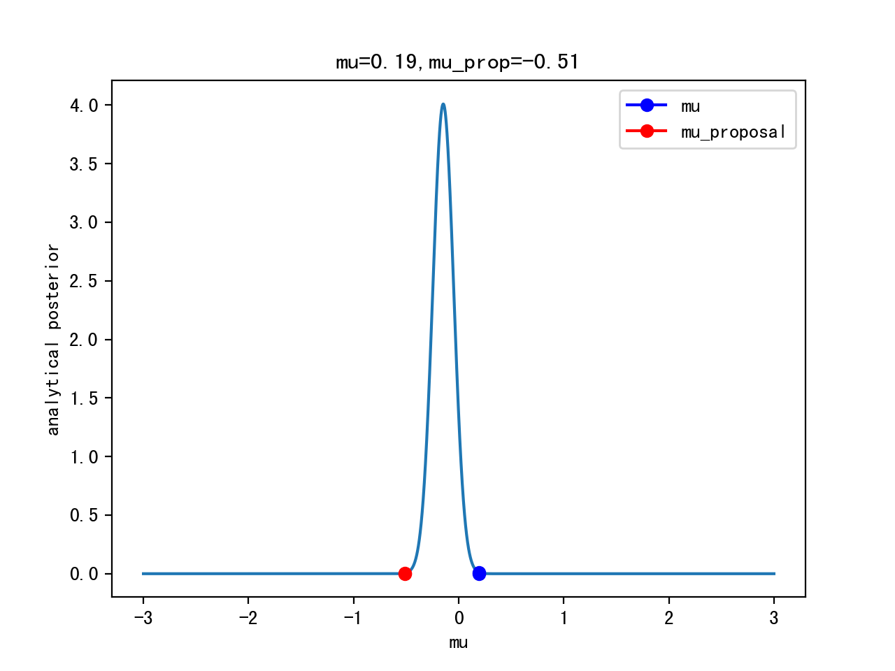
Iteration 1000:
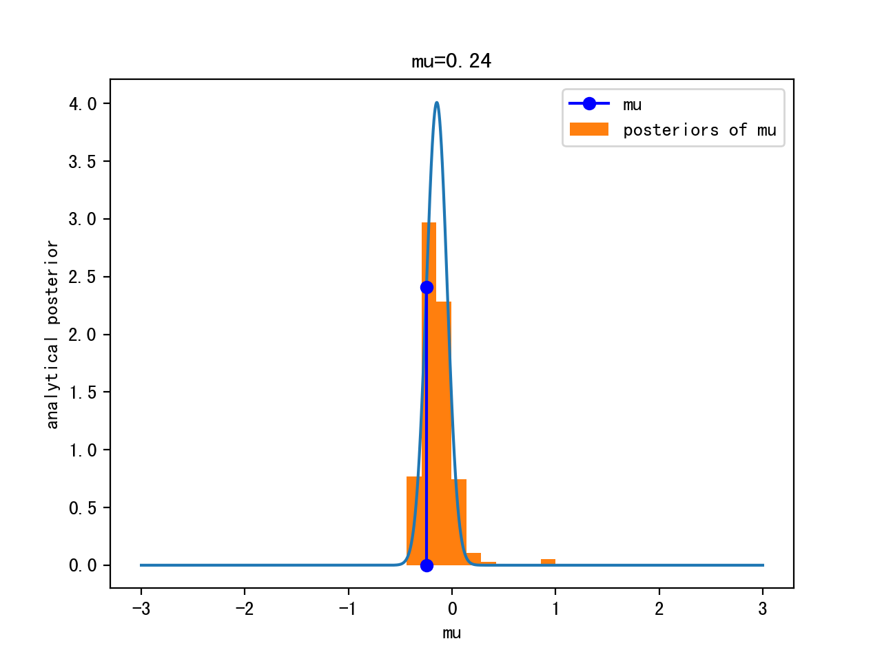
Iteration 10000:

Logistic Example
Summary
Suppose we want to sample from p(x), p(x) originally is Gaussian
Pre-requisite:
- assume log-probability of p(x) = -0.5*np.sum(x**2) without normalization constant
- determine proposal distribution: x’ ~ U(x-∆/2,x+∆/2)
- calculate p_acc: exp-log-p(x’)/exp-log-p(x)
- generate chain of x, calculate acceptance rate
Or, Given 100 data points, suppose we want to estimate the posterior of the mean p(θ|x)
Pre-requisite:
- assume a prior ~ Gaussian(ρ,τ), parameters known
- assume the likelihood based on data distribution ~ Gaussian(μ,σ), σ known for simplicity
- determine proposal distribution: Gaussian(μ,∆), ∆ known
- calculate p_acc: p(x|μ’)p(μ’)/p(x|μ)p(μ)
- generate chain of μ, calculate acceptance rate
In detail:
initialize μ
                    calc p(μ) fr prior G(ρ,τ)
  proposal       -> calc p(μ') fr prior G(ρ,τ) -                  lh(μ',σ|data)p(μ')
μ --------> μ' -|                               |--> calc p_acc = ------------------- -> μ=μ or μ'
                 -> calc likelihood fr G(μ,σ)  -                   lh(μ,σ|data)p(μ)
                    calc likelihood fr G(μ',σ)
References
Markov chain Monte Carlo (MCMC) sampling by Simeon Carstens
MCMC sampling for dummies
Markov Chain Monte Carlo in Python by Will Koehrsen
Markov Chain
Monte Carlo theory, methods and examples
Bayesian Methods for Hackers
