Restricted Boltzmann Machine
Energy-based Model
EBM defines a probability distribution through an Energy function
        exp(-E(x))      exp(-E(x))
p(x) = -----------  =  -----------
            Z          Σ exp(-E(x))
                       x

Z = Σ exp(-E(x))
    x
An EBM can be learned by performing SGD on the empirical negative log-likelihood of the training data
L(θ,D) = 1/N Σ    log p(x_i)   <- log-likelihood
             x_i∈D

l(θ,D) = - L(θ,D)   <- loss function

                        ∂log p(x_i)
stochastic gradient = - ------------
                             ∂θ

θ - model parameters
In many cases, we do not observe the example x fully, or we want to introduce some non-observed variables to increase the expressive power of the model
=> We consider an observed part x and a hidden part h:
                    exp(-E(x,h))
p(x) = Σ p(x,h) = Σ ------------
       h          h       Z
We define Free Energy:
F(x) = - log Σ exp(-E(x,h))
             h
Then:
        exp(-F(x))     exp(-F(x))
p(x) = ------------ = ------------
            Z         Σ exp(-F(x))
                      x

the negative       ∂log p(x)    ∂F(x)            ∂F(x~)
log-likelihood = - ---------- = ----- - Σ  p(x~) ------
gradient               ∂θ         ∂θ    x~         ∂θ

                 ∂F(x)
positive phase = -----
                  ∂θ
                            ∂F(x~)
negative phase = - Σ  p(x~) ------
                   x~         ∂θ
The terms ‘positive’ and ‘negative’ reflect their effect on the probability density defined by the model
Positive phase increases the probability of training data (by reducing the corresponding free energy)
Negative phase decreases the probability of samples generated by the model
the negative       ∂log p(x)    ∂F(x)               ∂F(x~)
log-likelihood = - ---------- ≈ ----- - 1/|N| Σ     ------
gradient               ∂θ         ∂θ          x~∈N    ∂θ

N - negative particles
where we could ideally like element x~ from N to be sampled according to p (i.e. Monte-Carlo)
The point is how to extract these negative particles N
The statistical literature abounds with sampling methods, i.e. MCMC + RBM
Boltzmann Machines
Boltzmann distribution aka Gibbs Distribution is from Thermodynamics, that’s why it’s called Energy-based Models.
Boltzmann Machines are a particular form of log-linear Markov Random Field (MRF), i.e. for which the energy function is linear in its free parameters.
To make them powerful enough to represent complicated distributions, we consider that some of the variables are never observed -> hidden variables (aka hidden units).
By having more hidden variables, we can increase the modeling capacity of the Boltzmann Machine.
Boltzmann Machines are models with only hidden and visible nodes:
- non-deterministic (stochastic)
- deep generative models
- unsupervised deep learning (only use inputs X, no labeling for the data)
No output nodes!
All the nodes are connected to all other nodes irrespective of whether they are input or hidden nodes.
This allows them to share information among themselves and self-generate subsequent data.
Restricted Boltzmann Machines
RBM restricts Boltzmann Machines to those without visible-visible and hidden-hidden connections
Two-layered NN with generative capabilities, which are connected by a fully bipartite graph
- visible layer (only connected to hidden layer)
- hidden layer (only connected to visible layer)
Bias units, the stochastic part, which is the different part from autoencoder
- visible bias - reconstruct the input during a backward pass
- hidden bias - produce the activation on the forward pass
(+) a symmetric bipartite graph
(+) multiple RBMs can be stacked and fine-tuned through GD and BP
(+) can learn a probability distribution
(-) being replaced by GAN or VA
RBM:
         o
   o  /  o
v  o --- o  h
   o  \  o
      W  o

   +     +
   a_i   b_j

v - visible layer (binary units)
h - hidden layer (binary units)
a - bias for v
b - bias for h
W - weights
Energy function:
E(v,h) = - h'Wv - a'v - b'h
       = - Σ Σ W * h * v - Σ a * v - Σ b * h
           j i |ji |j  |i  i |i  |i  j |j  |j
Free Energy:
F(v) = - Σ log Σ  exp(h_j(b_j+Wv))) - a'v
         j     h_j
Property of RBM:
visible and hidden units are conditionally independent given one-another
so we can write:
p(h|v) = ∏ p(h_j|v)
         j

p(v|h) = ∏ p(v_i|h)
         i
Distribution:
p(v,h) = exp ( -E(v,h) ) / Z

Z - partition function (intractable)
High-energy associated to low probability!!
RBMs with binary units
Binary units: v_i and h_j ∈ {0,1}
p(h_j=1|v) = sig (b_j+Wv)
p(v_i=1|h) = sig (a_i+hW')
The free energy can be:
F(v) = - Σ log (1+exp(b_j+Wv)) - a'v
         j
Then the gradients are:
  ∂log p(v)
- ---------- = E_v [p(h_j|v) * v_i] - v_ij * sig (Wv + b_j)
    ∂W_ij

  ∂log p(v)
- ---------- = E_v [p(h_j|v)] - sig (Wv)
    ∂a_i

  ∂log p(v)
- ---------- = E_v [p(v_i|h)] - v_ij
    ∂b_j

            exp(x)
sig(x) = ------------
          1 + exp(x)
Sampling:
Samples of p(x) can be obtained by running a Markov chain to convergence
Using Gibbs sampling as the transition operator
Can use Block Gibbs Sampling since visible and hidden units are conditionally independent:
A step in the Markov Chain is (n-th step):
h(n+1) ~ sig (Wv(n)+b)
v(n+1) ~ sig (h(n+1)W'+a)
As t->∞, samples (v(t),h(t)) are guaranteed to be accurate samples of p(v,h)
2 steps:
-
forward
h(1) = sig (Wv(0)+b) -
reconstruction (backward)
v(1) = sig (h(1)W'+a)
The Learning Process
v(0)-v(1) <- the reconstruction err we need to reduce in subsequent steps of the training process
In the forward pass
p(h(1)|v(0);W) - the probability of output h(1) given the input v(0) and the weights W
In the backward pass
p(v(1)|h(1);W)
Note: W in the forward/backward passes are the same
p(h|v;W) and p(v|h;W) lead to a joint distribution of inputs and the activations p(v,h)
Suppose the energy is given by E(v,h)
E(v,h) = - Σ a_i*v_i - Σ b_j*h_j - Σ v_i*h_j*w_ij
           i           j           i,j
           visible     hidden

v_i,h_j - the binary states of the visible unit i and hidden unit j
a_i,b_j - their biases
w_ij - the weights between them

p(v) = 1/Z Σ exp(-E(v,h))
           h

Z = Σ   exp(-E(v,h))
   v,h

       h
       Σ exp(-E(v,h))
p(v) = --------------
       Σ exp(-E(v,h))
      v,h
The log-likelihood gradient / the derivative of the log probability of a training vector w.r.t a weight is surprisingly simple:
∂log p(v)
--------- = <v_i*h_j>     - <v_i*h_j>
  ∂w_ij             |data           |model

<.> - expectations

Δw_ij = α (<v_i*h_j>     - <v_i*h_j>)
                   |data           |model

α - learning rate
Note:
- it’s easy to get an unbiased sample of <v_i*h_j>_data, because no direct connections between hidden units
- it’s difficult to get an unbiased sample of <v_i*h_j>_model, because it requires us to run a Markov chain until the stationary distribution is reached (which means the energy of the distribution is minimized - equilibrium!)
Instead of doing this, we can perform Gibbs Sampling from the distribution
Gibbs Sampling - an MCMC algorithm for obtaining a sequence of observations which are approximated from a specified multivariate probability distribution, when direct sampling is difficult
The Gibbs chain is initialized with a training sample v(0) and yields the sample v(k) after k steps
Each step t consists of sampling h(t) from p(h|v(t)) and sampling v(t+1) from p(v|h(t)) subsequently
v(0) -> h(t) ~ p(h|v(t)) -> v(t+1) ~ p(v|h(t)) -> v(k)
The learning rule becomes:
Δw_ij = α (<v_i*h_j>     - <v_i*h_j>)
                   |data           |recons
The learning works well even though it is only crudely approximating the gradient of the log probability of the training data.
The learning rule is much more closely approximating the gradient of another objective function called the Contrastive Divergence
Contrastive Divergence (CD-k) - the difference between two KL divergence:
                          ∂E(v_k,h)              ∂E(v_k,h)
CD(W,v(0)) = - Σ p(h|v_k) --------- + Σ p(h|v_k) ---------
  |k           h              ∂W      h              ∂W
where the second term is obtained after each k steps of Gibbs Sampling
The general intuition is that if parameter updates are small enough compared to the mixing rate of the chain, the Markov Chain should be able to ‘catch up’ to changes in the model.
RBM Implementation
Given MNIST binary data (60000x28x28 with only {0,1} values)
Train an RBM model with weights W, and bias a,b and generate learned samples
variable    dimension
 v∈{0,1}      784x1
 h∈{0,1}      100x1
    W         784x100
    a         784x1
    b         100x1

E(v,h) = - a'v    -    b'h     -     v'Wh
           / \         / \           /  \
      1x784x784x1    1x100x100x1   1x784x784x100x100x1

p(h=1|v) = sig(W'v+b)
               / \
            100x784x784x1
            100x1+100x1

p(v=1|h) = sig(Wh+a)
               /  \
             784x100x100x1
             784x1+784x1

h,v need to be sampled from p(h=1|v),p(v=1|h):
h ~ p(h=1|v)
v ~ p(v=1|h)

gradient update rule:
W += α(v0h0'-v1h1') 784x100
a += α(v0-v1) 784x1
b += α(h0-h1) 100x1

sig - element-wise sigmoid function
import numpy as np
import matplotlib.pyplot as plt

class RBM():

    def __init__(self,n_hid,n_vis):
        self.n_vis=n_vis
        self.n_hid=n_hid
        self.w=0.1*np.random.rand(self.n_vis,self.n_hid)
        self.a=0.1*np.random.rand(self.n_vis,1)
        self.b=0.1*np.random.rand(self.n_hid,1)
        self.alpha=0.01
        self.avg_energy_list=[]

    def sigmoid(self,z):
        return 1/(1+np.exp(-z))

    def forward(self,v):
        #p(h=1|v) = sig(W'v+b)  100x1=100x784x784x1+100x1
        h_dist=self.sigmoid(np.matmul(np.transpose(self.w),v)+self.b)
        return self.sample(h_dist)

    def backward(self,h):
        #p(v=1|h) = sig(Wh+a)  784x1=784x100x100x1+784*1
        v_dist=self.sigmoid(np.matmul(self.w,h)+self.a)
        return self.sample(v_dist)

    def sample(self,dist):
        n=dist.shape[0]
        true_idx=np.random.uniform(0,1,n).reshape(n,1) <= dist
        sampled=np.zeros((n,1))
        sampled[true_idx]=1
        return sampled

    def energy(self,v,h):
        #E(v,h) = - a'v - b'h - v'Wh
        return - np.inner(self.a.flatten(),v.flatten())-np.inner(self.b.flatten(),h.flatten()) -np.matmul(np.matmul(v.transpose(),self.w),h)

    def train(self,data,ep=10):
        data=data.reshape(data.shape[0],data.shape[1]*data.shape[2])
        #np.random.shuffle(data)
        for i in range(ep):
            self.energy_list=[]
            for j in range(data.shape[0]):
                v=data[j,:].reshape(-1,1) #784x1
                h_sampled=self.forward(v)
                v_sampled=self.backward(h_sampled)
                h_recon=self.forward(v_sampled)
                #W += alpha(v0h0'-v1h1') 784x100
                self.w += self.alpha*(np.matmul(v,np.transpose(h_sampled))-np.matmul(v_sampled,np.transpose(h_recon)))
                self.a += self.alpha*(v - v_sampled)
                self.b += self.alpha*(h_sampled - h_recon)

                self.energy_list.append(self.energy(v,h_recon))

            self.avg_energy_list.append(np.mean(self.energy_list))
            print('ep:'+str(i)+' data_idx:'+str(j)+' avg_energy:'+str(np.mean(self.energy_list)))

    def gibbs(self,n_iter=10,v_init=None):
        if v_init is None:
            v_init=np.random.rand(self.n_vis,1) #784x1

        v_t=v_init.reshape(-1,1) #784x1
        for i in range(n_iter):
            h_dist=self.sigmoid(np.matmul(np.transpose(self.w), v_t) + self.b)
            h_t=self.sample(h_dist)
            v_dist=self.sigmoid(np.matmul(self.w, h_t) + self.a)
            v_t=self.sample(v_dist)

        return v_t

if __name__=='__main__':
    #training
    mnist=np.load('mnist_bin.npy') #60000x28x28
    rbm=RBM(100,28*28) #n_hid 100, n_vis 784
    rbm.train(mnist[:200],ep=100)

    plt.plot(rbm.avg_energy_list)
    plt.savefig('avg_energy.png',dpi=350)

    #sampling
    #mnist figure 0~10
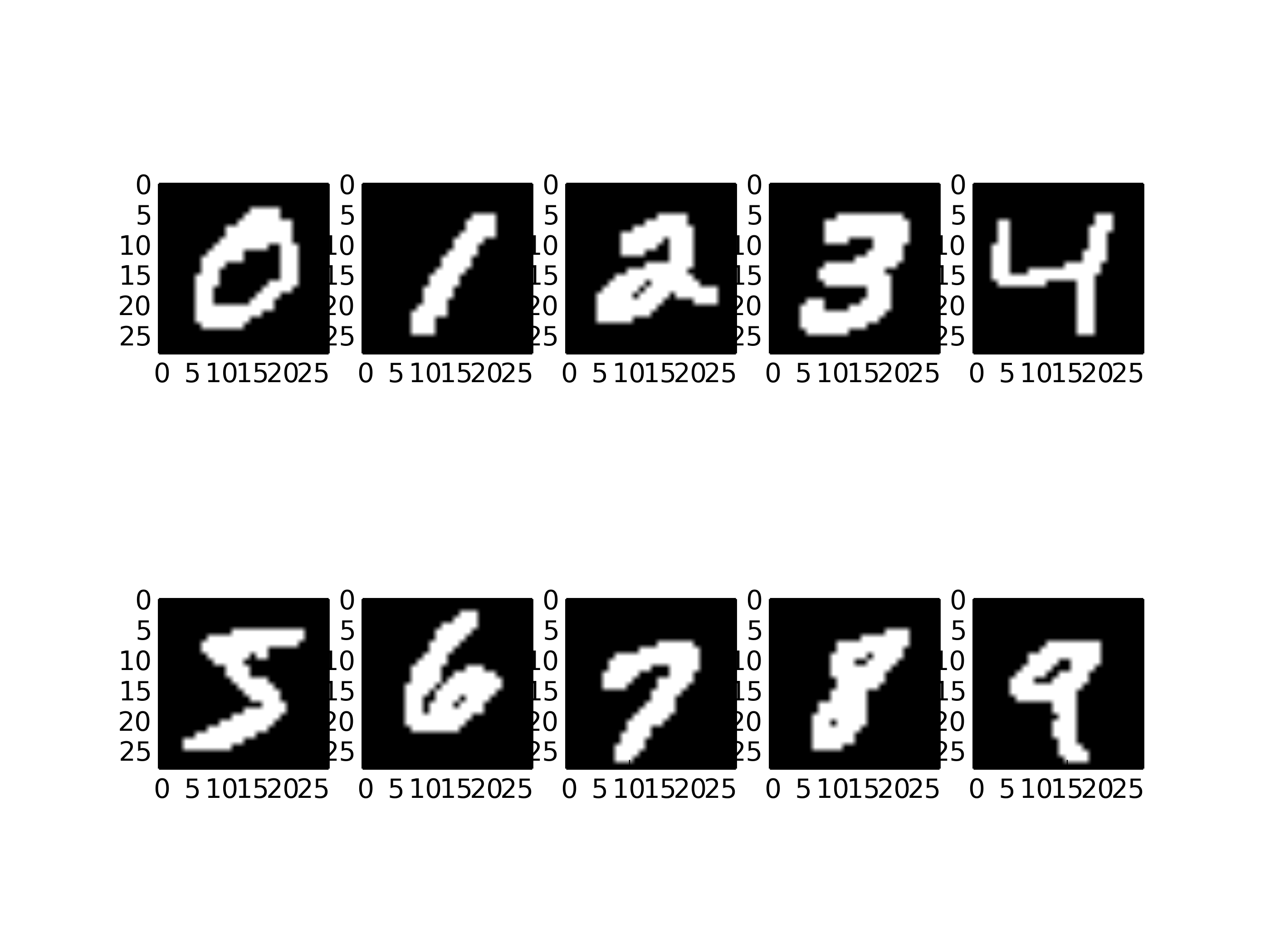
    mnist_idx=[1,3,5,7,2,0,13,15,17,4]
    plt.figure()
    for i in range(10):
        plt.subplot(2,5,i+1)
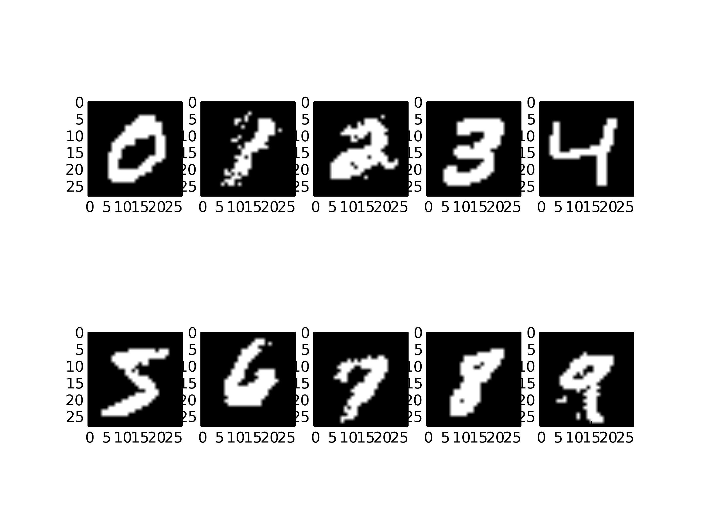
        v=rbm.gibbs(n_iter=1000,v_init=mnist[mnist_idx[i]])
        plt.imshow(v.reshape((28,28)),cmap='gray')

    plt.savefig('rbm_result.png',dpi=350)
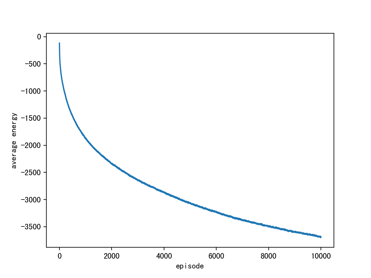
Results of hyperparameters:
episode length: 10000
sample size: 200x28x28
alpha: 0.1
Gibbs iterations: 1000
Average Energy:

Original mnist figure samples & Reconstructed samples:


In Summary:
Training process:
  forward
  training
v --------> h
|   W,a,b   |
v <-------- h
  backward
  training
Reconstruction using Gibbs sampling:
input: v_in, i.e. mnist figure '0'~'9'
output: v_out, reconstruction of v_in

     forward(v,w,b)   backward(h,w,a)
v_in -------------> h --------------> v -> ...... -> v_out
                                           n_iter
Applications
- dimensionality reduction
- classification
- regression
- collaborative filtering
- feature learning
- topic modeling
Unsupervised Learning
only use inputs X for learning
(+) automatically extract meaningful features for the data
(+) leverage the availability of unlabeled data
(+) add a data-dependent regularizer to training (-log p(X))
Algorithms:
- RBM
- autoencoder
- sparse coding model
Reference
RBM+mnist - github FengZiYjun
DeepLearning 0.1 documentation
Restricted Boltzmann Machine - Simplified
Bipartite graph - wiki
[1] LeCun, Yann, et al. “A tutorial on energy-based learning.” Predicting structured data 1.0 (2006).
