Importance Sampling

Definition

Consider a scenario for calculating an expectation of function f(x), where x~p(x)

E[f(x)] = ∫ f(x)p(x) dx ≈ 1/n Σ_n f(x_i)

The Monte Carlo sampling is to simply sample x from p(x), and take the average of all samples to get an estimation of the expectation

Problem:
What if p(x) is very hard to sample from?
Are we able to estimate the expectation based on some known and easily sampled distribution?

Say:

                                 p(x)                          p(x_i)
E[f(x)] = ∫ f(x)p(x) dx = ∫ f(x) ---- q(x) dx ≈ 1/n Σ_n f(x_i) ------
                                 q(x)                          q(x_i)

p(x) - the distribution hard to sample from
q(x) - the distribution easy to sample from
p(x)/q(x) - sampling ratio or sampling rate, which acts as a correction weight to offset the probability sampling from a different one

where x is sampled from q(x), (q(x) should not be 0)

By this way, estimating the expectation is able to sample from another distribution q(x)

Variance:

Var(X) = E[X^2] - E[X]^2

We need to avoid the situation when p(x)/q(x) is large (results in large variance), where X is f(x)p(x)/q(x)
We need to select proper q(x) that results in even smaller variance

python Example

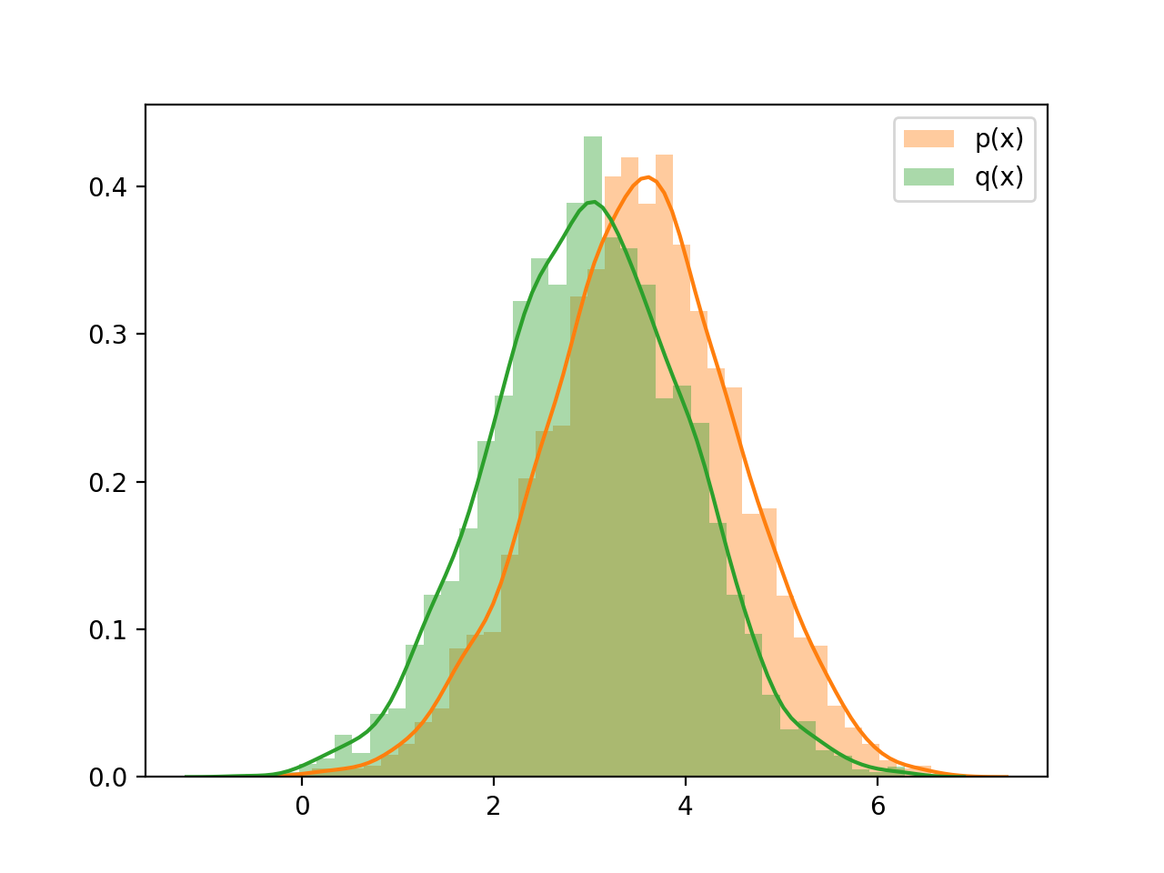
Draw two Gaussians with p=N(3.5,1), q=N(3,1), sample size=1000

import numpy as np
import matplotlib.pyplot as plt
from scipy.stats import norm
import seaborn as sns

def f(x):
    return 1/(1+np.exp(-x))

def dist(mu=0,sig=1):
    return norm(mu,sig)

n=1000
mu_tar=3.5
sig_tar=1
mu_app=3
sig_app=1

p=dist(mu_tar,sig_tar)
q=dist(mu_app,sig_app)

plt.figure()
sns.distplot([np.random.normal(mu_tar, sig_tar) for _ in range(3000)], label="p(x)")
sns.distplot([np.random.normal(mu_app, sig_app) for _ in range(3000)], label="q(x)")
plt.legend()

Sample from p(x), naively

v=[]
for i in range(n):
    x=np.random.normal(mu_tar,sig_tar) #sample from p(x)
    v.append(f(x))

np.mean(v)
>>0.9565661399403137
np.std(v)
>>0.04655246059295081

Sample from q(x), but with importance sampling

v=[]
for i in range(n):
    x=np.random.normal(mu_app,sig_app)  #sample from q(x)
    v.append(f(x)*p.pdf(x)/q.pdf(x))

np.mean(v)
>>0.9490444921104262
np.std(v)
>>0.5341476729005751

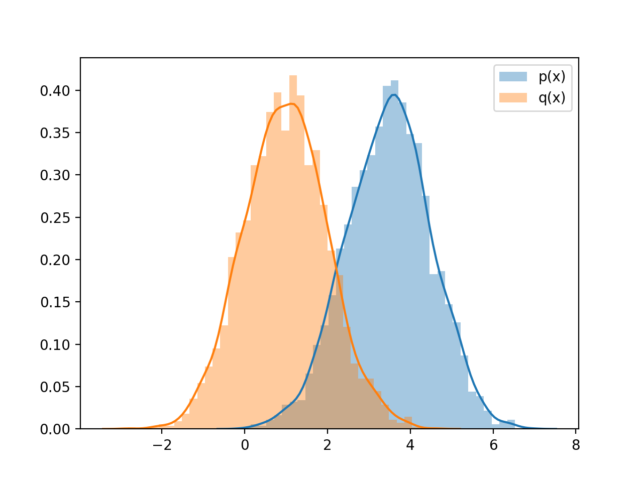
Try another q=N(1,1) with sample size=1000, increase sample size may help
the more different the distributions are , the more samples we need

n=1000
mu_app=1
sig_app=1

q=dist(mu_app,sig_app)
v=[]
for i in range(n):
    x=np.random.normal(mu_app,sig_app)  #sample from q(x)
    v.append(f(x)*p.pdf(x)/q.pdf(x))

np.mean(v)
>>1.0298267560057017
np.std(v)
>>14.146791278018734

Reference

Importance Sampling Introduction
Later check!
Metropolis and Gibbs Sampling