RL Dynamic Programming
Dynamic Programming in RL
DP here refers to algorithms that can be used to compute optimal policies given a perfect model of the env as MDP.
The key idea is the use of value functions to organize and structure the search for good policies
Assumption: MDP Dynamics is known
Goal: find optimal policy
(-) a perfect model needed
(-) they involve operations over the entire state set of the MDP
(-) computational expense
(-) hard to apply to continuous state and action spaces (very large) problems
(+) DP provides an essential foundation for understanding other RL methods
Notes:
A common way of obtaining approximate solutions for tasks with continuous states and actions is to quantize the state and action spaces, then apply finite-state DP methods.
Recall the Bellman Equations:
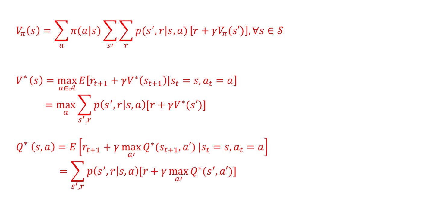
We can easily obtain optimal policies once we found the optimal value function V* or Q* which satisfy the Bellman optimality equations
Policy Evaluation
To compute Vπ by given π
Is concerned with making the state or action-values consistent with the current policy being followed
Iterative Policy Evaluation
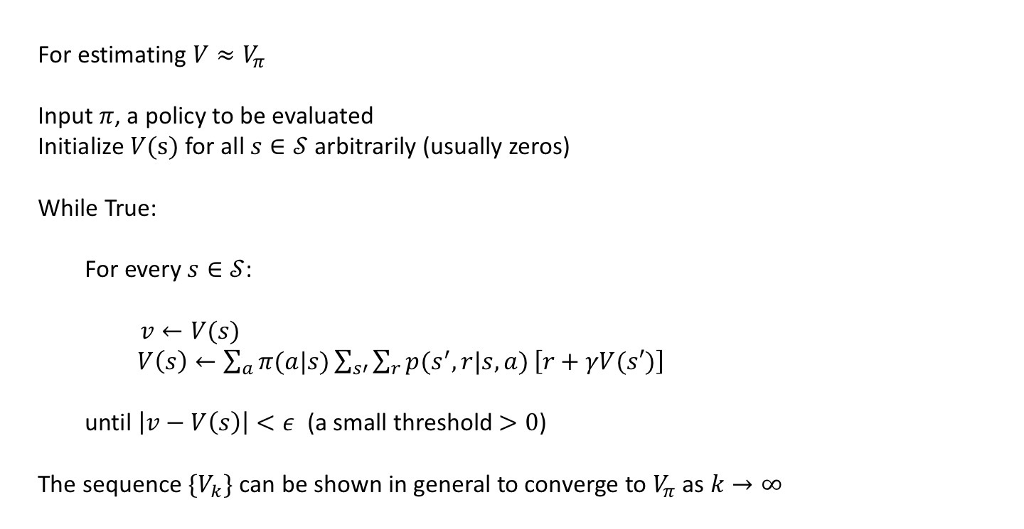
Expected Updates
based on an expectation over all possible next states rather than on a sample next state
Policy Improvement
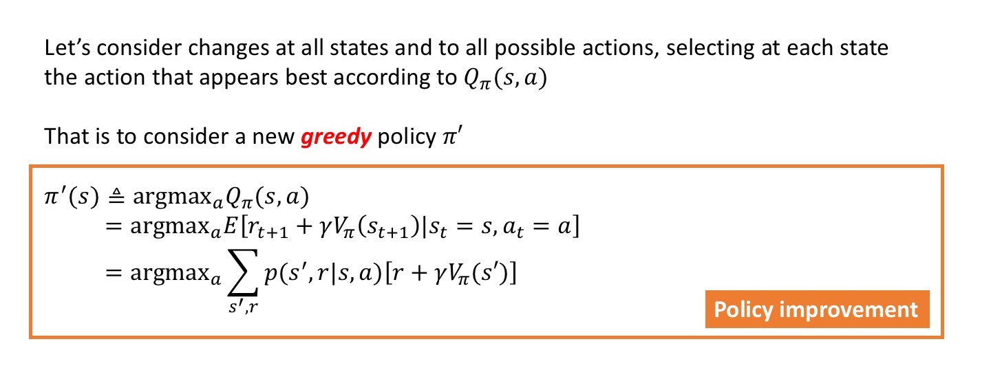
To find π’, a new policy by argmax_a Qπ(s,a)
Specifically, the process of making a new policy that improves on an original policy, by making it greedy w.r.t the value function of the original policy
Is concerned with adjusting the current policy to one that when followed leads to a higher return
Recall
Vπ(s) - how good it is to follow the current policy from s
The reason to compute Vπ is to find better policies
How to determine if it is better to change to the new policy?
Use Qπ(s,a) - selecting a in s following policy π
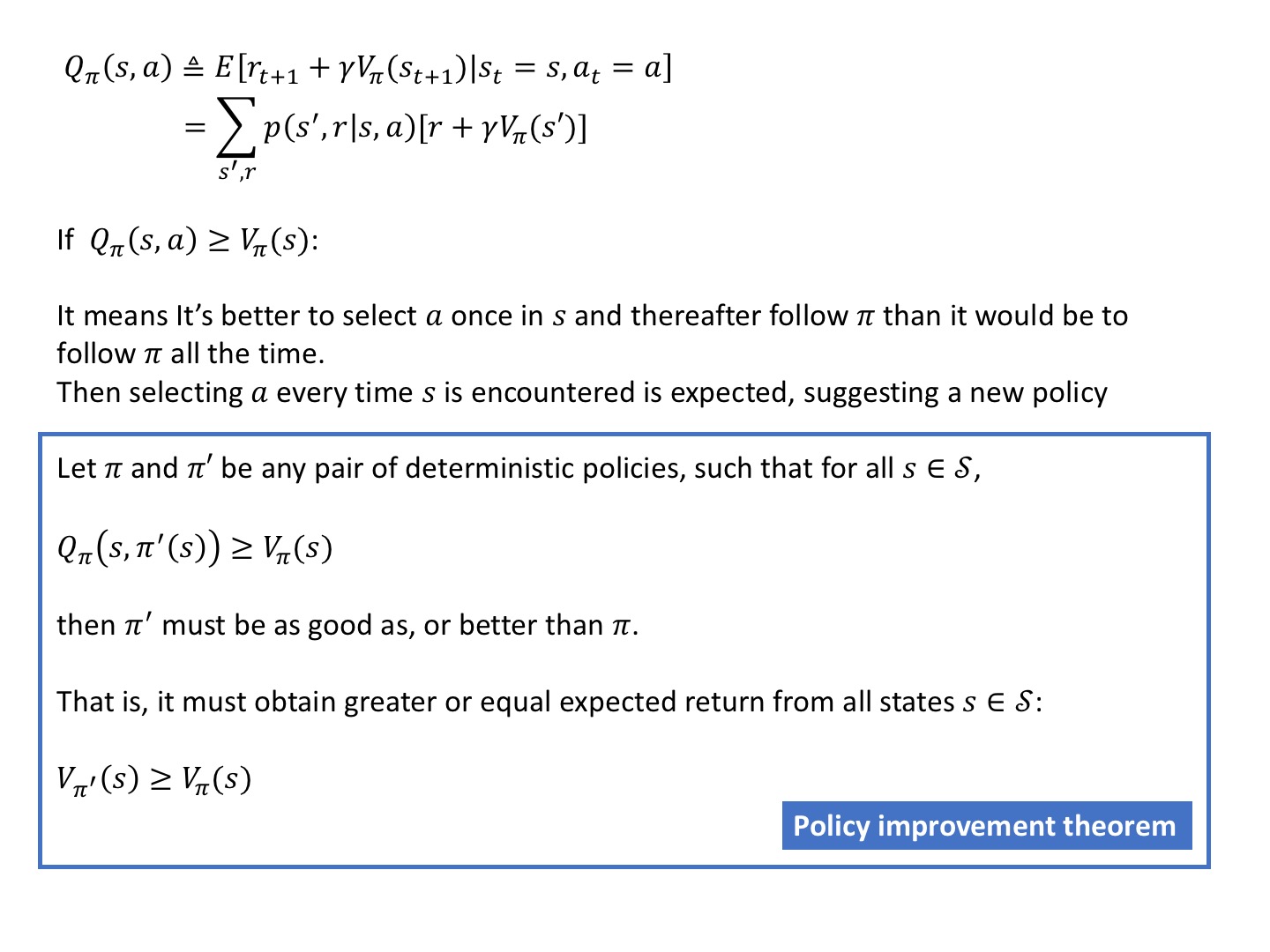
Given a policy π and it’s value functions Vπ and Qπ, we can evaluate a change in the policy at a single state to a particular action
Example 4.1 GridWorld - python, implementation of Policy Evaluation
deterministic: p(s'|s,a)=1     Episodic Task

  ----|---|---|----         terminal states: ///
  |///| 1 | 2 | 3 |         actions={up,down,left,right}
  |---|---|---|---|         if out of grid, leave its location unchanged
  | 4 | 5 | 6 | 7 |         reward:
  |---|---|---|---|             r=-1 on all transitions until the terminal state is reached
  | 8 | 9 | 10| 11|
  |---|---|---|---|         gamma=1 <- undiscounted
  | 12| 13| 14|///|
  ----|---|---|----         compute the Vπ(s), π(s,a)=0.25 - uniform random
                            Vπ(s)=sum(π*[r+gamma*V(s')]) along actions
         4X4                record π(s) of argmaxVπ(s)
import numpy as np

nA,nX,nY=4,4
actions=[[0,-1],[-1,0],[0,1],[1,0]] #left,up,right,down
pi=0.25
gamma=1

def is_terminal(s):
    return (s[0]==0 and s[1]==0) or (s[0]==nX-1 and s[1]==nY-1)

def step(s,a):
    if is_terminal(s):
        return s,0

    s_=[s[0]+a[0],s[1]+a[1]]
    if s_[0]<0 or s_[0]>=nX or s_[1]<0 or s_[1]>=nY:
        s_=s

    r=-1
    return s_,r

v=np.zeros((nX,nY))
pi_op=np.zeros((nX,nY))
iter=0
while True:
    v_new=np.zeros_like(v)
    for x in range(nX):
        for y in range(nY):
            vs=[]
            for i,a in enumerate(actions):
                (x_,y_),r=step([x,y],a)
                vs.append(pi*(r+gamma*v[x_,y_]))
            v_new[x,y]=np.sum(vs)
            pi_op[x,y]=np.argmax(vs)
    if np.sum(np.abs(v-v_new))<1e-4:
        print(np.round(v,decimals=3))
        print(pi_op)
        print(iter)
        break
    v=v_new
    iter+=1

>>V
[[  0. -14. -20. -22.]
 [-14. -18. -20. -20.]
 [-20. -20. -18. -14.]
 [-22. -20. -14.   0.]]

>>pi_op    #argmax can only find the first occurance index
[[0. 0. 0. 0.]
 [1. 0. 3. 3.]
 [1. 2. 2. 3.]
 [1. 2. 2. 0.]]
'''
[[l. l. l. l.]
 [u. l. d. d.]
 [u. r. r. d.]
 [u. r. r. l.]]
'''
>>iter:217
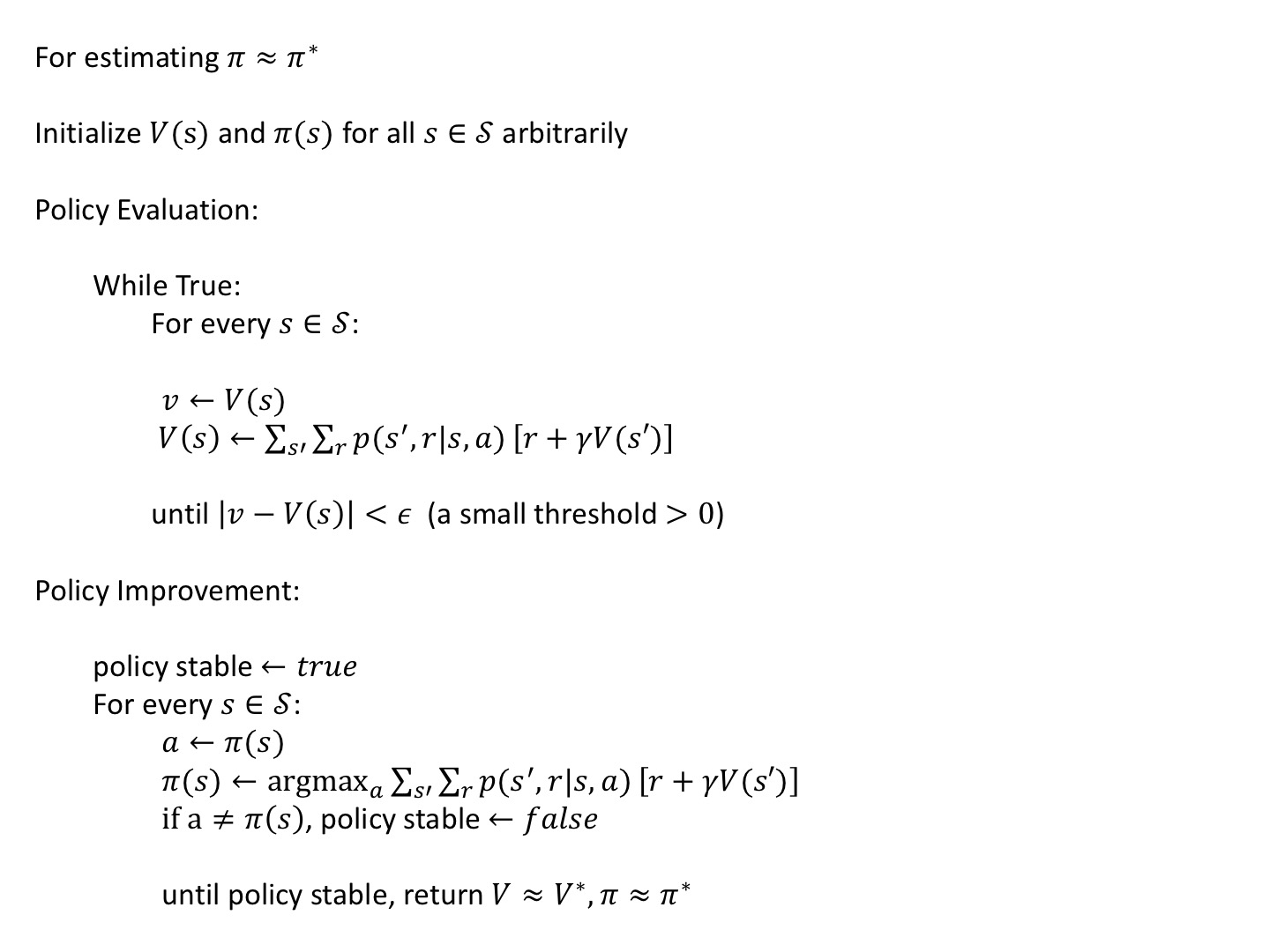
Policy Iteration
To find optimal π* with the help of finding Vπ*
π0 -> Vπ0 -> π1 -> Vπ1 -> ... -> π* -> Vπ*
   PE     PI    PE     PI     PI    PE
PE - Policy Evaluation
PI - Policy Improvement
Policy Iteration results in faster convergence than Policy Evaluation, presumably because the value function changes little from one policy to the next
Value Iteration
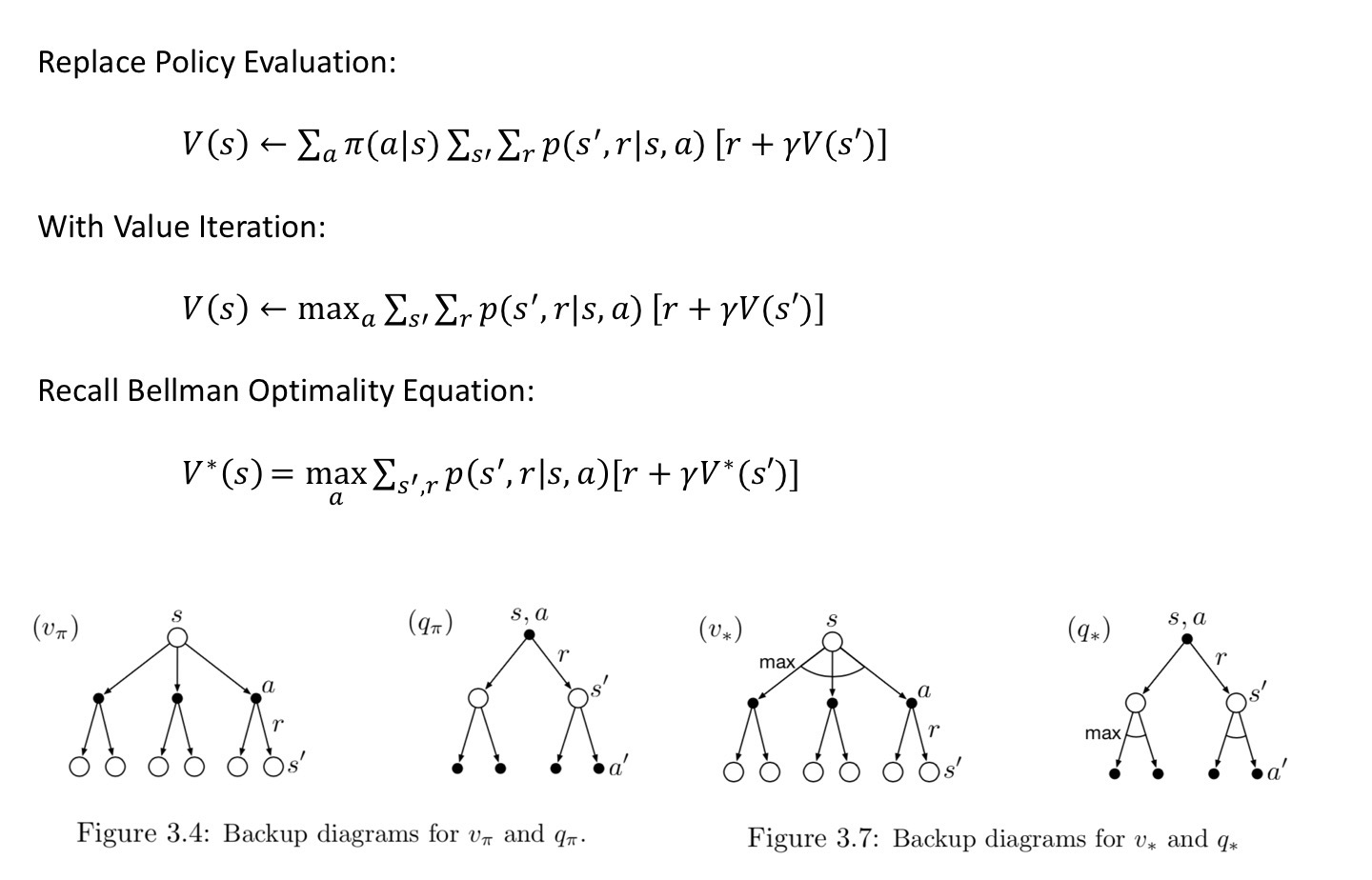
Update V(s) with max_a ∑∑p(s’,r|s,a)[r+𝛾V(s’)]
Drawback of Policy Iteration:
(-) each of its iterations involves policy evaluation, which may itself be protracted iterative computation requiring multiple sweeps through the state set
Solution:
It may be possible to truncate policy evaluation without losing the convergence guarantees of policy iteration
Ways of viewing Value Iteration
- in each of VI’s sweeps, one sweep of PE and one sweep of PI
- Value Iteration is obtained simply by turning the Bellman Optimality Equation into an update rule
- compare backup diagrams of Vπ and V*
- the max operation is added to some sweeps of policy evaluation
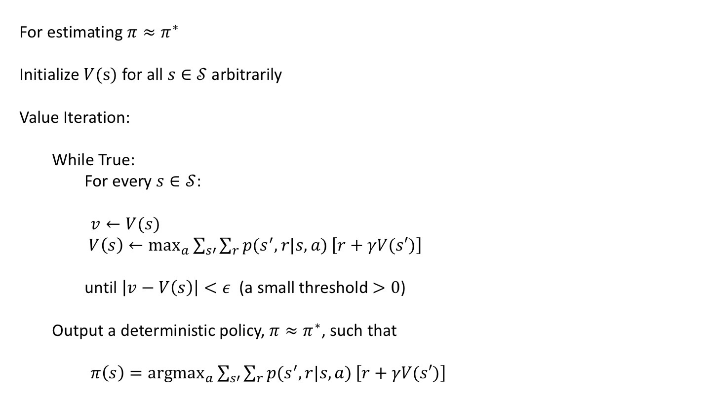
All of these algorithms converge to an optimal policy for discounted finite MDPs
Value Iteration VS Policy Iteration
Recall:
In Policy Iteration each of its iterations involves policy evaluation, which may itself be protracted iterative computation requiring multiple sweeps through the state set
However,
In Value Iteration, with the max operator, it needs to consider all actions
Policy Iteration computes the value for some fixed policy π(s)
It can start with an arbitrary policy π0, and repeat until the policy converges
Policy Iteration Complexity:
Time: O(|S|^3+|A||S|^2)
Space: O(|S|)
Q-Value Iteration
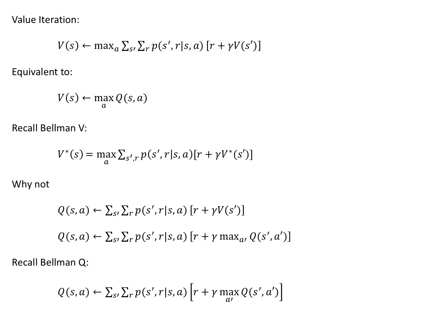
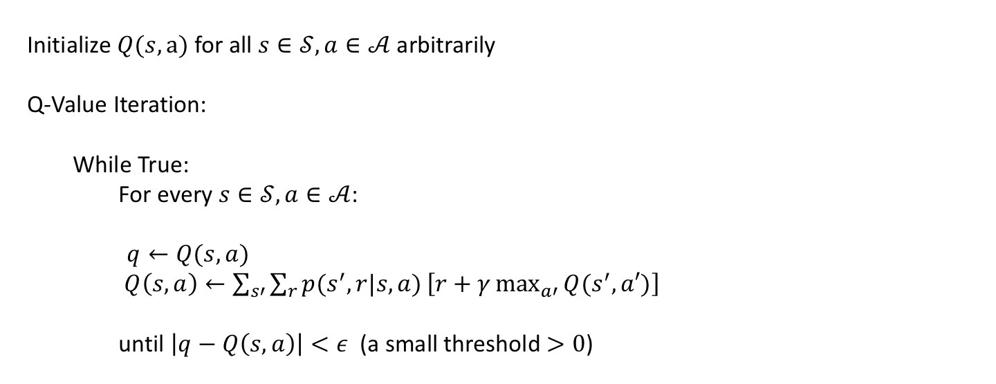
Example 4.1 GridWorld - python, implementation of Value Iteration and Q-Value Iteration
deterministic: p(s'|s,a)=1     Episodic Task

  ----|---|---|----         terminal states: ///
  |///| 1 | 2 | 3 |         actions={up,down,left,right}
  |---|---|---|---|         if out of grid, leave its location unchanged
  | 4 | 5 | 6 | 7 |         reward:
  |---|---|---|---|             r=-1 on all transitions until the terminal state is reached
  | 8 | 9 | 10| 11|
  |---|---|---|---|         gamma=1 <- undiscounted
  | 12| 13| 14|///|
  ----|---|---|----         compute the V*(s) and Q*(s,a)
                            V(s)=max([r+gamma*V(s')]) along actions
         4X4                Q(s,a)=r+gamma*max(Q(s',a'))
                            record π(s) of argmax_a Vπ(s), argmax_a Q(s,a)
#Valute Iteration
v=np.zeros((nX,nY))
pi_op=np.zeros_like(v)
iter=0
while True:
    v_new=np.zeros_like(v)
    for x in range(nX):
        for y in range(nY):
            vs=[]
            for i,a in enumerate(actions):
                (x_,y_),r=step([x,y],a)
                vs.append(r+gamma*v[x_,y_])
            v_new[x,y]=np.max(vs)
            pi_op[x,y]=np.argmax(vs)
    if np.sum(np.abs(v-v_new))<1e-4:
        print(np.round(v,decimals=3))
        print(pi_op)
        print(iter)
        break
    v=v_new
    iter+=1

#q-value iteration
def sub2num(x,y):
    return x*nX+y

def num2sub(n):
    return [n//nX,n%nY]

N=nX*nY
q=np.zeros((N,nA))
n,n_=0,0
iter=0
while True:
    q_new=np.zeros_like(q)
    for x in range(nX):
        for y in range(nY):
            qs=[]
            for i,a in enumerate(actions):
                (x_,y_),r=step([x,y],a)
                n=sub2num(x,y)
                n_=sub2num(x_,y_)
                qs.append(q[n_,i])
            q_new[n,a]=r+gamma*max(qs)
    if np.sum(np.abs(q-q_new))<1e-4:
        q_max=np.max(q,axis=1)
        a_max=np.argmax(q,axis=1)
        v_out=np.zeros((nX,nY))
        a_out=np.zeros((nX,nY))
        for j in range(N):
            a,b=num2sub(j)
            v_out[a,b]=q_max[j]
            a_out[a,b]=a_max[j]
        print(np.round(v_out,decimals=3))
        print(np.round(a_out,decimals=3))
        print(cnt)
        break
    q=q_new
    iter+=1

>> #V of Value Iteration
[[ 0. -1. -2. -3.]
 [-1. -2. -3. -2.]
 [-2. -3. -2. -1.]
 [-3. -2. -1.  0.]]
>> #pi_op
[[0. 0. 0. 0.]
 [1. 0. 0. 3.]
 [1. 0. 2. 3.]
 [1. 2. 2. 0.]]
>>iter:3

>> #V=maxQ(s,a) of Q-Value Iteration
[[0. 0. 0. 0.]
 [0. 0. 0. 0.]
 [0. 0. 0. 0.]
 [0. 0. 0. 0.]]
>> #a=argmaxQ(s,a)
[[0. 2. 2. 2.]
 [2. 2. 2. 2.]
 [2. 2. 2. 2.]
 [2. 2. 2. 0.]]
>>iter:1
Asynchronous DP
One Drawback of DP:
(-) they involve operations over the entire state set of the MDP
Asyn DPs are in-place iterative DPs that are not organized in terms of systematic sweeps of the state set
They updates the values of states in any order whatsoever, using whatever values of other states happen to be available
(+) flexibility
(+) help the agent not get locked into any hopeless long sweep before it can make progress
(+) make it easier to intermix computation with real-time interaction
(-) still need to continue to update the values of all the state
To solve a given MDP, we can run an iterative DP at the same time that an agent is actually experiencing the MDP. The agent’s experience can be used to determine the states to which the DP applies its updates.
Generalized Policy Iteration
To find optimal policy π* and optimal value function V*
Refer to the general idea of letting Policy Evaluation and Policy Improvement processes interact, independent of the granularity and other details of the two processes
The value function only stabilizes when it is consistent with the current policy, and the policy stabilizes only when it is greedy with respect to the current value function
Efficiency of DP
Let |S| and |A| denote the number of states and actions
A DP is guaranteed to find an optimal policy in polynomial time, even the total number of (deterministic) policy is |A|^|S|
Comparable methods which can solve MDPs:
- Dynamic Programming
- Linear Programming
References
Sutton’s RL book second edition, Chapter 4 Dynamic Programming
shangtongzhang github
