Bellman Equation
finite MDP
MDPs are a classical formalization of sequential decision making, where actions influence not just immediate rewards, but subsequent situations, or states, and through those future reward
Thus MDPs involve delayed reward and the need to tradeoff immediate and delayed reward
In Bandit Problems:
- estimate the Q*(a) of each action
In MDPs:
- estimate the Q*(s,a) of each action in each state, or
- estimate the V*(s) of each state given optimal action selections
Basic Formulation and Return
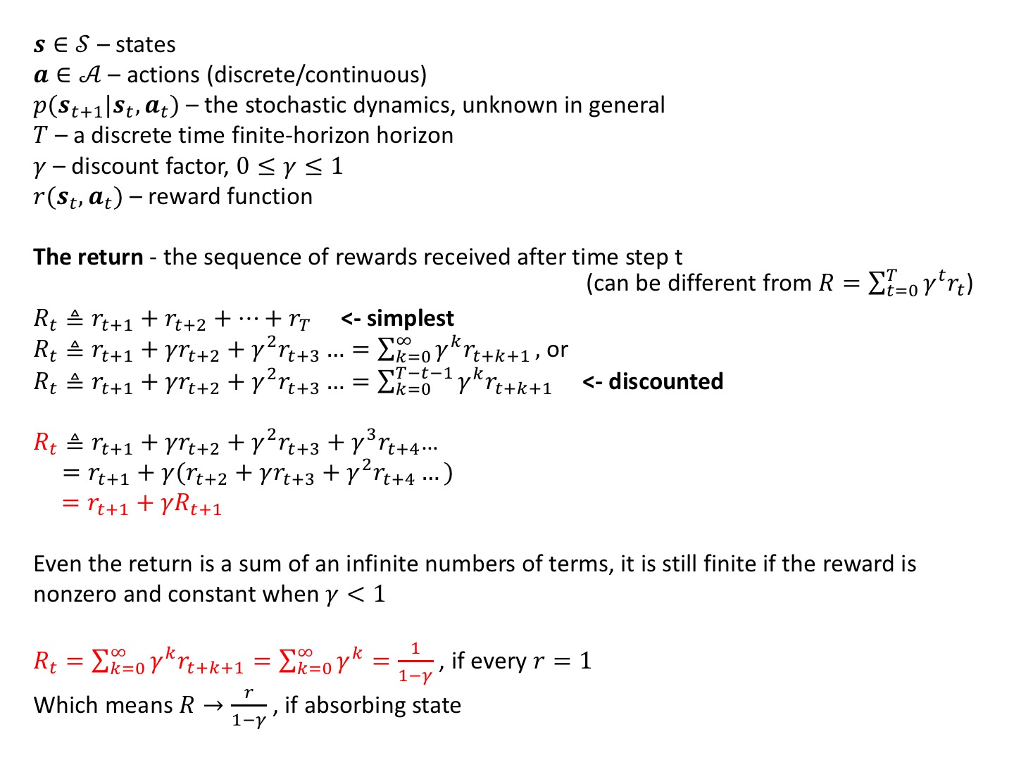
Episodic and Continuing tasks
Episodic: the agent-env interaction naturally breaks down into a sequence of separate episodes
(+) mathematically easier because each action affects only the finite number of rewards subsequently received during the episode
Markov Property
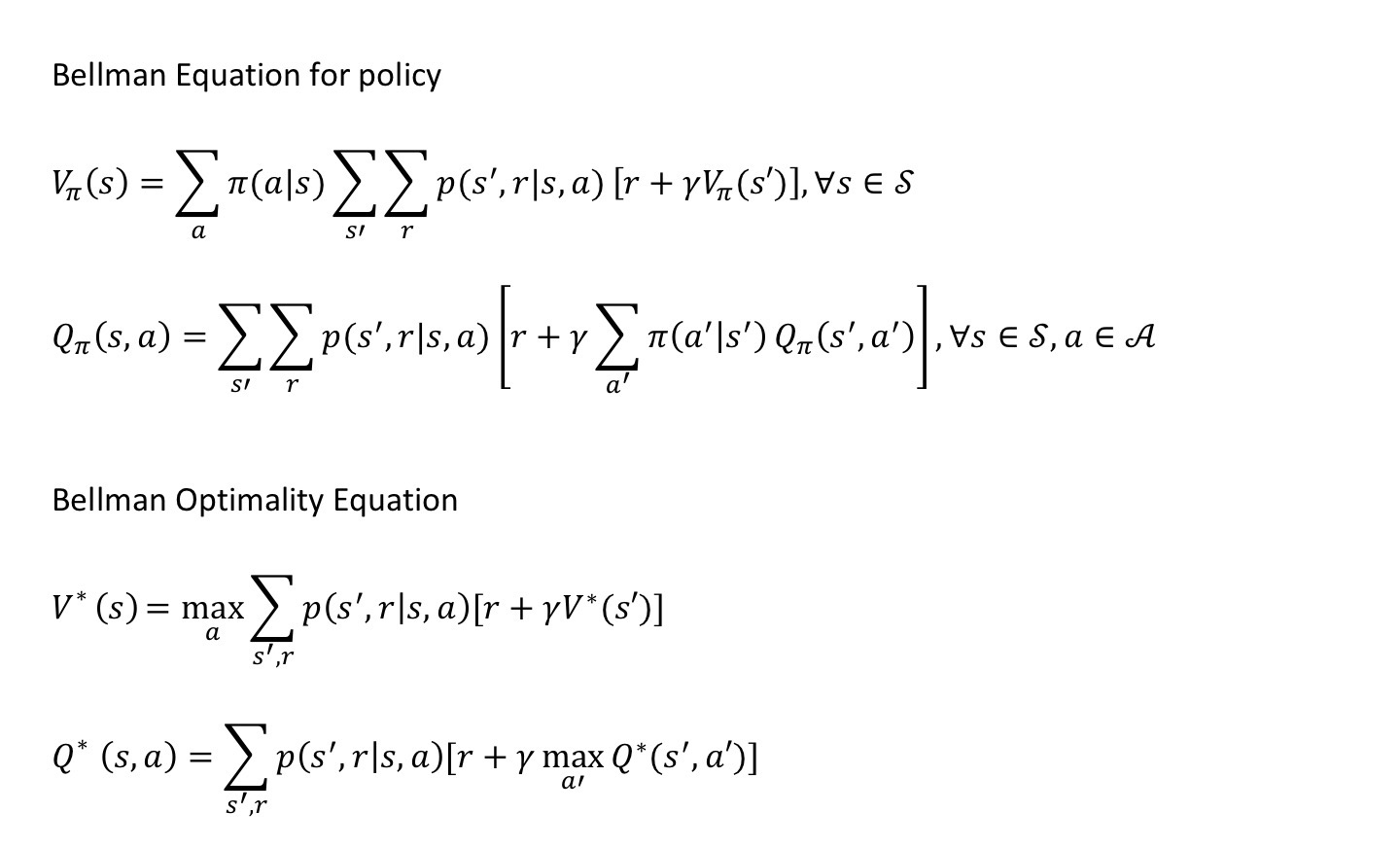
Bellman Equation
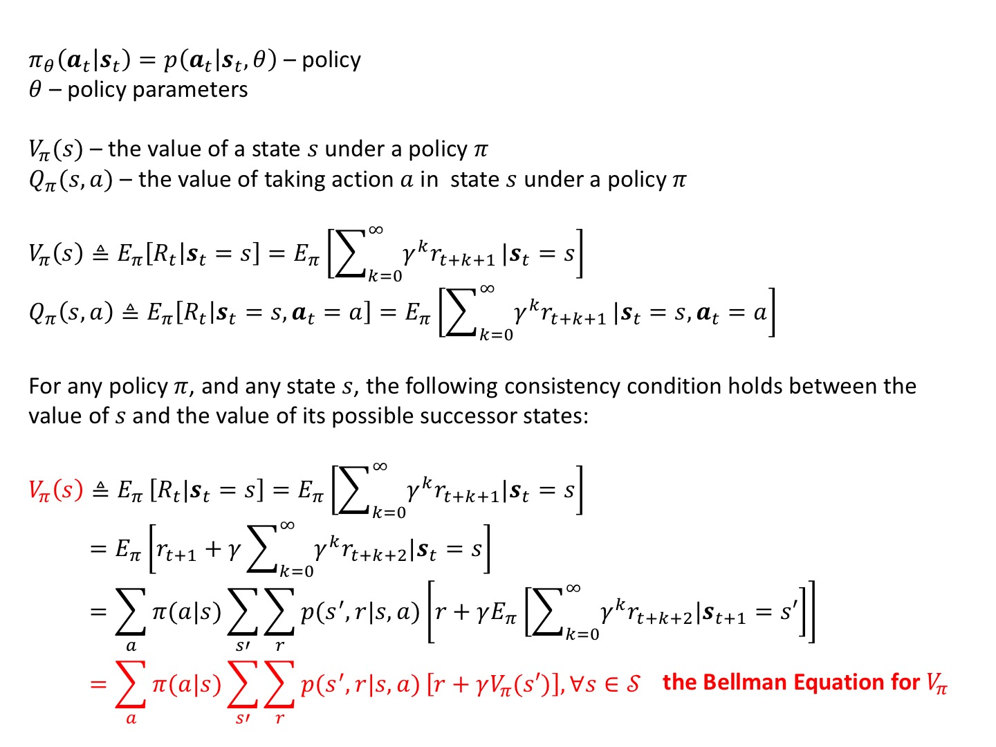
Value Function
“How Good” it is for the agent to be in a given state, or
“How Good” it is to perform a given action in a given state in terms of expected return
Value function are defined w.r.t particular policies, that is the rewards the agent can expect to receive in the future depend on what actions it will take
- V and Q can be estimated from experience, such as Monte Carlo methods
- V and Q can be maintained as parameterized functions by the agent, and the parameters can be adjusted to better match the observed returns
- V and Q satisfy particular recursive relations which is Bellman Equation <- fundamental property
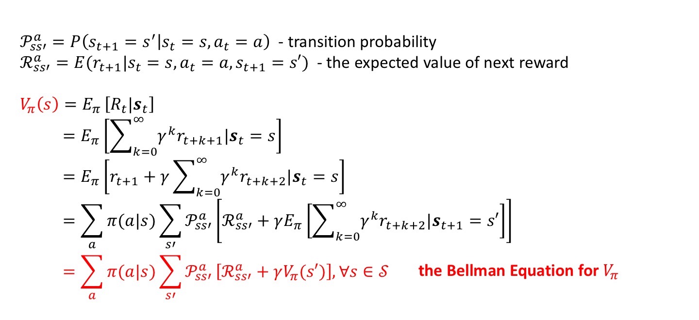
Bellman Equation
- expresses a relationship between the value of a state and the values of its successor states
- averages over all the possibilities, weighting each by its probability of occurring
- states that the value of the start state must equal the (discounted) value of the expected next state, plus the reward expected along the way
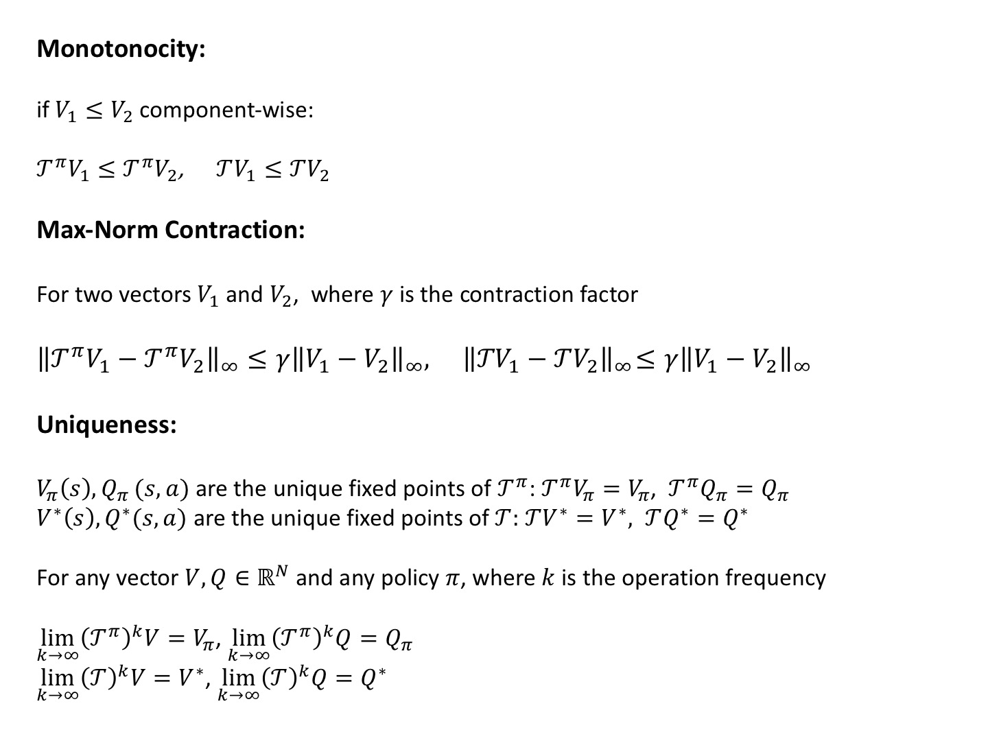
The value function V is the unique solution to its Bellman equation
Monte Carlo methods
averaging over many random samples of actual returns
Example 3.5 GridWorld - python
use Bellman Equation to compute the value matrix until convergence
deterministic: p(s'|s,a)=1      Continuing Task
----|---|---|---|----
|   | A |   | B |   |        actions={up,down,left,right}
|---|---|---|---|---|        reward:
|   |   |   |   |   |          out of grid: r=-1, leave its location unchanged
|---|---|---|---|---|          state A-> state A': r=+10
|   |   |   | B'|   |          state B-> state B': r=+5
|---|---|---|---|---|          others: r=0
|   |   |   |   |   |        pi(a|s)=1/#actions=0.25
|---|---|---|---|---|        gamma=0.9
|   | A'|   |   |   |        compute the V(s) based on bellman equation
----|---|---|---|----        V(s)=sum(pi*[r+gamma*V(s')]) along action
         5X5
Solution:
from state [0,0], apply 4 actions, get 4 new_state, and 4 rewards
compute the sum of all pi*[r+gamma*V(s’)] for V(s)
state - action - new_state - reward   -  V(s)=pi*(r+gamma*V(newS))
[0,0]   [0,-1]   [0,0]         -1        0.25*(-1+0.9*V[0,0])=-0.25
[0,0]   [-1,0]   [0,0]         -1        0.25*(-1+0.9*V[0,0])=-0.25
[0,0]   [0,1]    [0,1]         0         0.25*(0+0.9*V[0,1])=0
[0,0]   [1,0]    [1,0]         0         0.25*(0+0.9*V[1,0])=0
                                         sum up to V[0,0]=-0.5
[0,1]
[0,2]
[0,3]
  :
  :
[4,0]
[4,1]
[4,2]
[4,3]
[4,4]
start over, until convergence
import numpy as np
nX,nY=5,5
pos_A=[0,1]
pos_A_=[4,1]
pos_B=[0,3]
pos_B_=[2,3]
actions=[[0,-1],[-1,0],[0,1],[1,0]] #left,up,right,down
pi=0.25
gamma=0.9

def step(s,a):
    if s==pos_A:
        return pos_A_, 10
    if s==pos_B:
        return pos_B_, 5

    s_=[s[0]+a[0],s[1]+a[1]]
    if s_[0]<0 or s_[0]>=nX or s_[1]<0 or s_[1]>=nY:
        r=-1
        s_=s
    else:
        r=0

    return s_,r

v=np.zeros((nX,nY))
while True:
    v_new=np.zeros_like(v)
    for x in range(nX):
        for y in range(nY):
            vs=[]
            for a in actions:
                (x_,y_),r=step([x,y],a)
                vs.append(pi*(r+gamma*v[x_,y_]))
            v_new[x,y]=np.sum(vs)
    if np.sum(np.abs(v-v_new))<1e-4:
        print(v)
        break
    v=v_new
    #replace v with v_new cuz v should remain same at each round of action averaging

>>
[[ 3.30903373  8.78932925  4.42765654  5.32240493  1.49221608]
 [ 1.52162547  2.99235524  2.25017731  1.90760904  0.54744003]
 [ 0.05085989  0.73820797  0.67315062  0.35822355 -0.40310382]
 [-0.97355491 -0.43545805 -0.35484491 -0.58556775 -1.18303775]
 [-1.85766316 -1.34519388 -1.2292299  -1.42288081 -1.97514172]]

>>iter:76
Bellman Optimality Equation
If the dynamics of the environment are known, in principle one can solve this system of equations for V* using any one of a variety of methods for solving systems of nonlinear equations
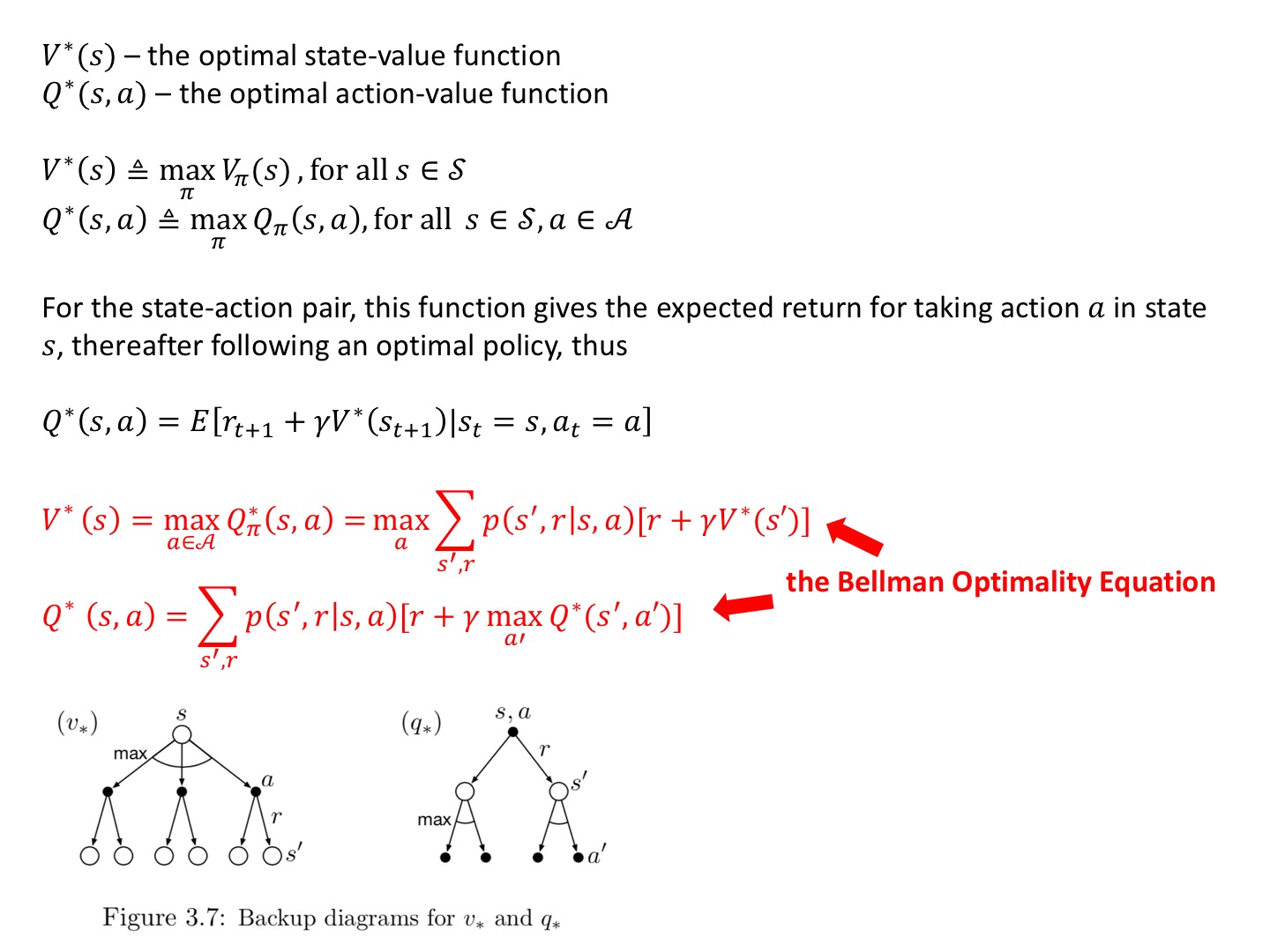
Because it is the optimal value function, however, V*’s consistency condition can be written in a special form without reference to any specific policy
Bellman Optimality Equation
- expresses the fact that the value of a state under an optimal policy must equal the expected return for the best action from that state
Example 3.8 GridWorld - python Value Iteration use the Bellman Optimality Equation to compute V*
Solution:
Other than Example 3.5 using uniform policy, the policy here is unknown
Every time we compute V(s)=max of all [r+gamma*V(s’)] along actions
v=np.zeros((nX,nY))
while True:
    v_new=np.zeros_like(v)
    for x in range(nX):
        for y in range(nY):
            vs=[]
            for a in actions:
                (x_,y_),r=step([x,y],a)
                vs.append(r+gamma*v[x_,y_])
            v_new[x,y]=np.max(vs)
    if np.sum(np.abs(v-v_new))<1e-4:
        print(v)
        break
    v=v_new

>>
[[21.97744338 24.41938153 21.97744338 19.41938153 17.47744338]
 [19.77969904 21.97744338 19.77969904 17.8017056  16.02153504]
 [17.8017056  19.77969904 17.8017056  16.02153504 14.41938153]
 [16.02153504 17.8017056  16.02153504 14.41938153 12.97744338]
 [14.41938153 16.02153504 14.41938153 12.97744338 11.67969904]]

>>iter:123
Bellman Operator
Recall
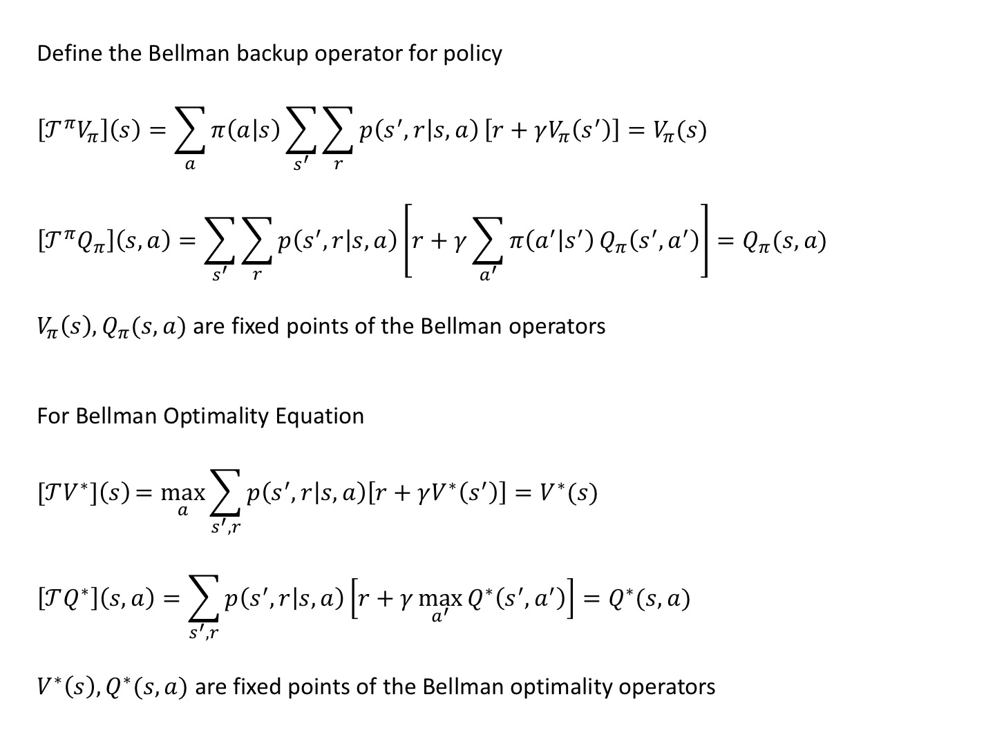
Bellman Operator Properties
References
Sutton’s RL book second edition, Chapter 3 Finite MDPs
shangtongzhang github
Previous Edition